This article was previously published in Computer Physics Communications, 110088 (Kabus, et al., 2026). More about Pigreads can be found online at its code repository on GitLab, its documentation. A PDF of the article can be downloaded at the website of Computer Physics Communications 110088 (DOI: 10.1016/j.cpc.2026.110088), or directly here.
Authors:
Desmond Kabus1,2 (ORCID: 0000-0002-6965-5211)
Hans Dierckx1,2 (ORCID: 0000-0003-0899-8082)
Tim De Coster1,2 (ORCID: 0000-0002-4942-9866)
Institutions:
Laboratory of Experimental Cardiology, Leiden University Medical Center (LUMC), Albinusdreef 2, 2333 ZA Leiden, The Netherlands
Mathematical Institute, Leiden University, Einsteinweg 55, 2333 CC Leiden, The Netherlands
DOI: 10.1016/j.cpc.2026.110088
Keywords:
- reaction-diffusion
- finite differences
- Python
- OpenCL
- GPU
- electrophysiology
Highlights:
- GPU-accelerated reaction-diffusion solver in up to three dimensions.
- Minimal NumPy-friendly API with OpenCL kernels.
- Includes commonly used reaction terms for cardiac electrophysiology.
- Open-source, tested, documented, with examples and tutorials.
Abstract:
Pigreads is a streamlined Python module for efficient numerical solution of reaction-diffusion systems on graphics cards (GPU), with CPU fallback. It exposes a simple and straight-forward NumPy-compatible API. Users may employ built-in models – including electrophysiology examples – or supply custom reaction terms. Supported features include 0D-3D uniform Cartesian grids, no-flux and periodic boundary conditions, anisotropic diffusion, spatially varying diffusion and reaction, and localised source terms. The project is open-source, tested, documented, and distributed with examples and tutorials.
Introduction
Reaction-diffusion systems appear across physics, chemistry, biology, and ecology; they are used to study pattern formation and excitable waves, for instance in electrophysiology (Cannon et al., 2014; Clayton et al., 2011; Kapral & Showalter, 1995; Lechleiter et al., 1991; Murray, 1976; Rotermund et al., 1990). Their numerical solution can be computationally demanding, so efficient implementations are essential, ranging from ad-hoc research codes to large general software packages (Niederer et al., 2011). However, modern applications such as inverse problems, parameter estimation, uncertainty quantification, and machine learning, require a compact code with minimal installation requirements that is portable across platforms, runs fast, and can easily be integrated into other software or frameworks.
Pigreads is a Python module (van Rossum et al., 1995) that provides a minimal, concise, and NumPy-friendly API (Harris et al., 2020) to define and run reaction-diffusion simulations while performing the costly computations efficiently on accelerators: Computational kernels implemented in OpenCL (Stone et al., 2010) run on both GPUs and CPUs as a fallback via PyOpenCL (Klöckner et al., 2012). The Pigreads module includes several pre-defined models relevant to electrophysiology; users can also supply custom reaction terms.
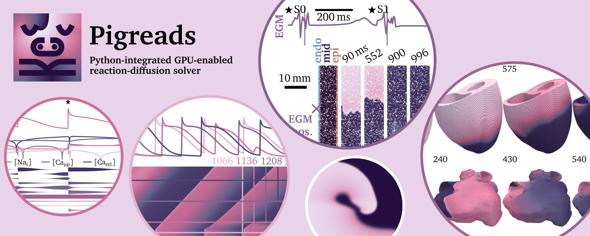
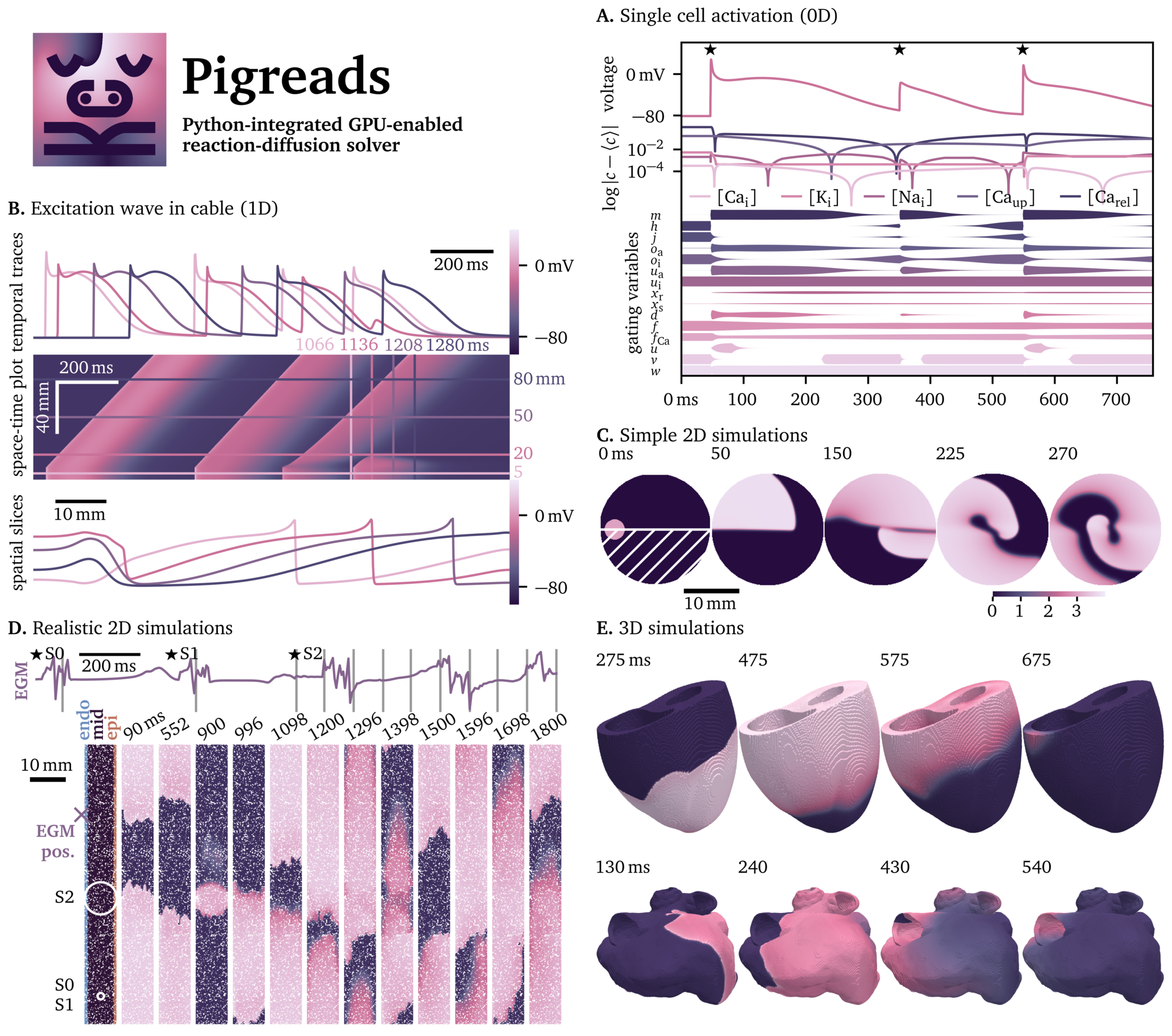
Representative examples are illustrated in Fig. 1: simulations of the conduction in a 1D cable of excitable cells, 2D pieces of cardiac tissue like monolayers in culture wells, and numerical electrophysiology experiments of whole organs in 3D like the ventricles or atria of the human heart. The 0D case, i.e., without diffusion, is also supported to perform single cell simulations.
The module is available on GitLab, where it is properly tested using continuous integration, and is well-documented on Read the Docs, with examples and tutorials. Pigreads can be installed from the Python Package Index PyPI via:
$ pip install pigreads
Consider also installing the optional dependencies for the command line interface (CLI) and creating plots and videos via:
$ pip install 'pigreads[all]'
The CLI can be used to run and visualise Pigreads simulations defined in a YAML file (Net, 2023) adhering to a Pydantic scheme as described in the documentation.
Mathematical problem definition
We generally define reaction-diffusion systems as:
$$
\partial_t {{\underline{{u}}}}(t, {{\bm{{x}}}})
=
\underbrace{
{{\underline{{P}}}} \nabla \cdot {{\bm{{D}}}}({{\bm{{x}}}}) \nabla {{\underline{{u}}}}(t, {{\bm{{x}}}})
}_{\text{diffusion}}
+
\underbrace{
{{\underline{{r}}}}({{\underline{{u}}}}, {{\bm{{x}}}})
}_{\text{reaction}}
+
\underbrace{
{{\underline{{s}}}}(t, {{\bm{{x}}}})
}_{\text{source}}
\qquad{(1)}$$ for time
$t\in[0, T]$ and space
${{\bm{{x}}}} = {{{{\left[ x, y, z \right]}}}^\mathrm{T}} \in\heartsuit\subset\mathbb R^3$
in the domain $\heartsuit$, with initial conditions
${{\underline{{u}}}}(0, {{\bm{{x}}}})$ and no-flux
boundary conditions
$0 = {{\bm{{n}}}}\cdot {{\bm{{D}}}} \nabla u$ for
diffused variables on
${{\bm{{x}}}} \in \partial\heartsuit$. At each point
in time and space, the states vector
${{\underline{{u}}}}(t, {{\bm{{x}}}}) \in \mathbb R^{\mathtt{Nv}}$
consists of Nv elements, the so-called states or variables,
$u_0$, $u_1$, …,
$u_{\mathtt{Nv}-1}$. For the diffusion term, we
define the diffusivity matrix ${{\bm{{D}}}}({{\bm{{x}}}}) \in
\mathbb R^{3\times 3}$ and the selection matrix
${{\underline{{P}}}} \in \mathbb
R^{\mathtt{Nv}\times\mathtt{Nv}}$ to select which variables to
diffuse and how strongly. The selection matrix often takes the sparse
form ${{\underline{{P}}}} =
\operatorname{diag}(P_{0}, ..., P_{\mathtt{Nv}-1})$ with
mostly zeros. The reaction term
${{\underline{{r}}}}({{\underline{{u}}}}, {{\bm{{x}}}}) \in \mathbb R^{\mathtt{Nv}}$
describes the local dynamics of the system and may vary in space, for
instance in parameters or even in the model equations themselves. We
refer to a specific local choice of
${{\underline{{r}}}}_{\mathtt{imodel}}({{\underline{{u}}}})$
with fixed parameters as a model;
${{\underline{{r}}}}$ refers to the reaction term,
i.e., all models. The source term
${{\underline{{s}}}}(t, {{\bm{{x}}}}) \in \mathbb R^{\mathtt{Nv}}$
can be used to add external influences to the system, for instance to
stimulate the system at specific times and locations.
For no source term, ${{\underline{{s}}}} = 0$, homogeneous and isotropic diffusion, ${{\bm{{D}}}}({{\bm{{x}}}}) = D = \text{const.}$, and only two variables, $u = u_0$ and $v = u_1$, with only $u$ diffusing, $P_0 = 1$, $P_1 = 0$, the system reduces to: $$ \begin{align} \partial_t u(t, {{\bm{{x}}}}) &= D \nabla^2 u(t, {{\bm{{x}}}}) + r_u(u, v) \\ \partial_t v(t, {{\bm{{x}}}}) &= r_v(u, v) \end{align} \qquad{(2)}$$
Technical overview
Pigreads organises simulation components around three objects: an
instance of the class Models that defines local reaction terms, an
array inhom that defines the domain and which model to use where, and
an array states holding all state variables on a uniform Cartesian
grid; see also the flowchart in Fig. 2.
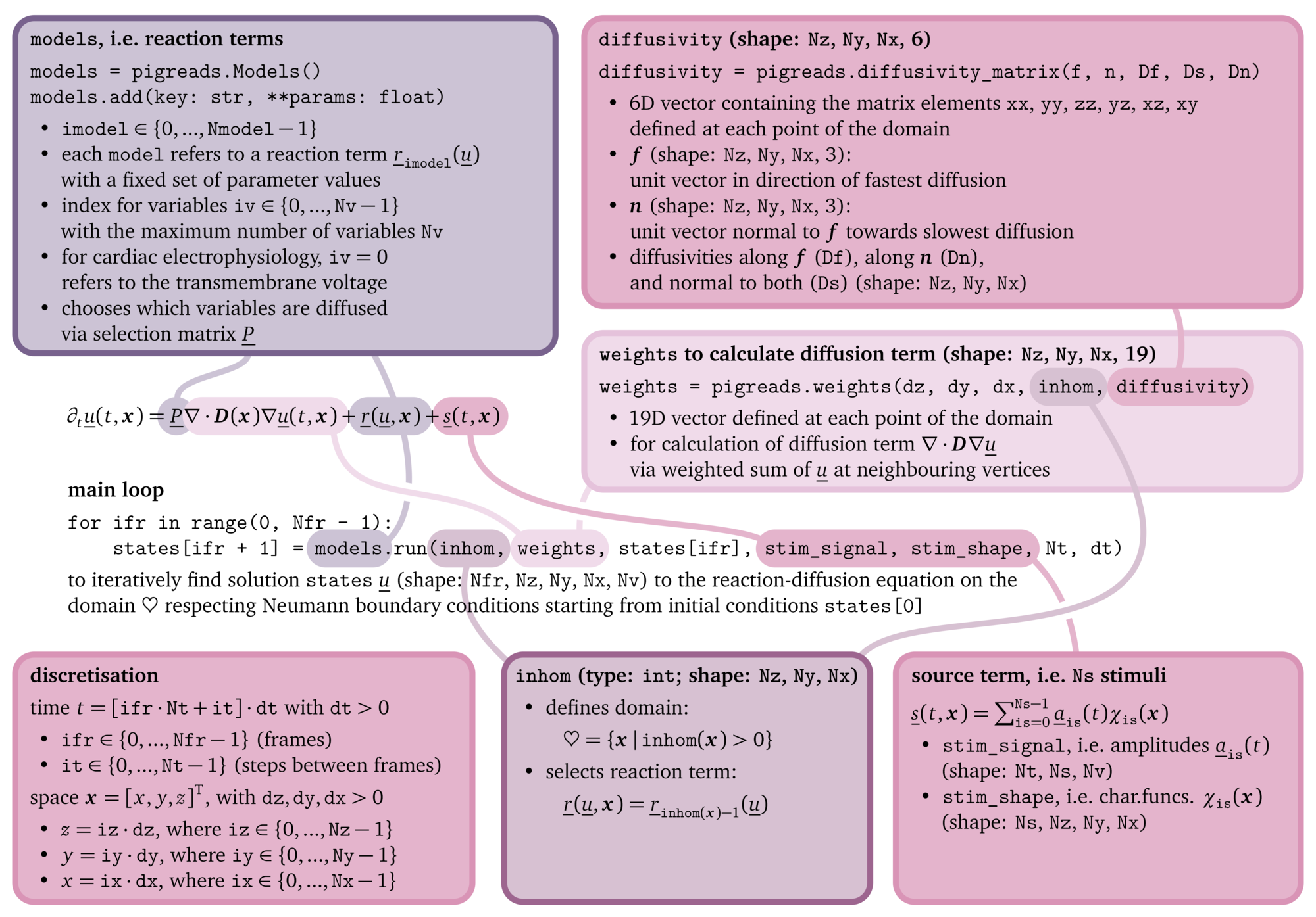
Figure 2: Main components of a simulation to solve a
reaction-diffusion problem using Pigreads. The state variables at each
point in the grid at the frames are stored in the variable states. The
main computations are done in the method models.run, which performs
Nt forward Euler steps with time step dt, outputting the subsequent
frame after these Nt steps.
Numerical choices are deliberately simple: finite-difference stencils for spatial derivatives and explicit forward-Euler time stepping. Supported capabilities include 0D-3D grids, no-flux and periodic boundary conditions, spatially varying anisotropic diffusivity and reaction terms, and source terms.
Diffusion and reaction kernels run in OpenCL on the selected GPU/CPU device; Python performs setup, parameter changes, and in- and output while results remain accessible as NumPy arrays for analysis and plotting, for instance using Matplotlib (Hunter, 2007) or PyVista (Sullivan & Kaszynski, 2019).
Note that execution of the kernels requires a compatible OpenCL runtime environment. For example, for Nvidia graphics cards, the runtime is provided through the CUDA toolkit and corresponding device drivers. For AMD devices, it is available via the AMD ROCm platform, and for Intel devices, through the Intel oneAPI toolkit. Alternatively, the PoCL implementation can be used for CPU-based or generic OpenCL execution.
We validated our code by using it to successfully compute the correct solution to the problem proposed by Niederer et al. (2011): simulation of the model by ten Tusscher & Panfilov (2006) for 100 ms in a slab of 3 × 7 × 20 mm. As a benchmark, on an NVIDIA GeForce RTX 2080 Super GPU with Max-Q Design, the computations take 0.025 s at the coarsest resolution of 0.5 mm and 0.05 ms; and 41.9 s at the finest resolution of 0.1 mm and 0.005 ms.
Unit testing is used to ensure all components of Pigreads work as expected: Code changes are automatically tested using continuous integration where the API is exercised and numerically validated against known results. The tests cover 100% of the code.
Hands-on example
In this section, we define and run a simple 2D simulation of a spiral wave in a two-variable model that breaks up to spiral chaos in a circular domain with no-flux boundary conditions. With this example, it is shown in which steps a Pigreads simulation is usually defined.
First, define the coordinates of the geometry to be used. In this example, we use a 2D plane with 200 points in both $x$ and $y$:
import pigreads as pig
import numpy as np
R = 10
z, y, x = np.mgrid[0:1, -R:R:200j, -R:R:200j]
Nz, Ny, Nx = x.shape
dz, dy, dx = pig.deltas(z, y, x)
Pigreads is optimised for three-dimensional space. For lower-dimensional
simulations, set the number of points in additional dimensions to one,
as done above for the $z$-dimension. Note that
np.mgrid is used to define a dense multi-dimensional grid where the
coordinates, in this case, are defined as the range of integers from 0
up to but excluding 1 in z, i.e., $z \in \{0\}$,
and -R to R divided into 200 equal steps including both end points
in y and x. See the documentation of NumPy for details. The function
pig.deltas returns the grid spacing dz, dy, dx that is used in
the arrays z, y, x, which each have a shape of (Nz, Ny, Nx).
Space in Pigreads is periodic by default, such that the points at index
ix = 0 are neighbours with the points at ix = 1 and ix = Nx - 1,
and likewise for the other dimensions.
The grid spacing dz, dy, dx must be chosen small enough to resolve
the dynamics of the system, but large enough to keep the computational
cost manageable. For instance, at insufficient spatial resolution, the
conduction is slower along grid axes than diagonal to them. One may use
this effect to determine an as large as possible grid spacing dx such
that the difference between the fastest and slowest stimulation at some
distance is less than a given threshold, for instance 5%.
The integer field inhom defines which points are outside
(inhom == 0) and inside the domain $\heartsuit$
(inhom > 0). Pigreads implements no-flux boundary conditions on
$\partial\heartsuit$. In our example, we define the
domain $\heartsuit$ as a disk of radius
$R$:
inhom = np.ones(x.shape, dtype=int)
r = np.linalg.norm((x, y, z), axis=0)
inhom[r >= R] = 0
Values of inhom larger than zero can be used to select one or multiple
models, i.e., reaction terms ${{\underline{{r}}}}$.
For an inhom value of 1, models[0] is used; and models[1] for a
value of 2, etc. One or more of the available models can be selected
using an instance of the Models class:
models = pig.Models()
models.add("marcotte2017dynamical", beta=1.389)
Nv = models.Nv
The key of a model – an identifying string – is here used to choose
a model and keyword arguments are used to set model parameters to
different values than the defaults; the function add may be called
multiple times to add more models. When using multiple models, the
largest number of variables Nv is used.
Various models are pre-defined in Pigreads, and defining another model is straight-forward, see section 5. A list of the available models can also be obtained programmatically using:
for key in pig.Models.available.keys():
    print(key)
# aliev1996simple
# barkley1991model
# beeler1977reconstruction
# ...
For some models, there are multiple sets of parameters available, they
may be accessed via the additional meta data of a model definition:
key = "tentusscher2006alternans"
model_def = pig.Models.available[key]
endo = model_def.meta["parameter sets"]["endo"]
for parameter, value in endo.items():
    print(f"{parameter} = {value}")
# g_Ks = 0.392
# g_to = 0.073
# s_offset = 28.0
# s_variant = 1.0
models_ = pig.Models()
models_.add(key, **endo)
In the next step, memory needs to be allocated to store the state
variables of the model. For this, we typically use a 5D array of shape
(Nfr, Nz, Ny, Nx, Nv) called states in Pigreads. It consists of the
values of all Nv variables at each point in space on Nfr so-called
frames in time.
One way to initialise a states array is using the function
models.resting_states: It creates an array of the correct shape and
fills its first frame with the appropriate resting values for each model
according to the value of inhom:
Nfr = 100
states = models.resting_states(inhom, Nframes=Nfr)
assert states.shape == (Nfr, Nz, Ny, Nx, Nv)
Note that this allocates a potentially large amount of memory, as
states is a 5D array of shape (Nfr, Nz, Ny, Nx, Nv). For large
simulations, it may be better to only store a few frames and overwrite
older frames, or to save frames to disk and not keep them in memory, for
instance via memory mapping:
states = np.lib.format.open_memmap("states.npy",
    mode='w+', dtype=np.float32,
    shape=(Nfr, Nz, Ny, Nx, Nv),
)
states[:1] = models.resting_states(inhom, Nframes=1)
If the full history over time does not need to be kept, it is also
possible to create a states array of only a few frames, continually
overwriting them in an infinite loop. We use this scheme in some of the
interactive examples that can be found in the code repository.
Initial conditions can then be set in the frame with ifr = 0:
states[0, x < -8, 0] = 1
states[0, y < 0, 1] = 2
Or equivalently expressed in mathematical notation: $$ \begin{align} u_0(t = 0, {{\bm{{x}}}}) &= \begin{cases} 1 & \text{if}\, x < -8 \\ u_{0,\,\text{rest}} & \text{else} \end{cases} \\ u_1(t = 0, {{\bm{{x}}}}) &= \begin{cases} 2 & \text{if}\, y < 0 \\ u_{1,\,\text{rest}} & \text{else} \end{cases} \end{align} \qquad{(3)}$$
The calculation of the diffusion term
${{\underline{{P}}}} \nabla \cdot
{{\bm{{D}}}} \nabla {{\underline{{u}}}}$ is implemented as a
weighted sum of neighbouring points. The weights can be calculated using
the function weights, which also requires the diffusivity
${{\bm{{D}}}}$ as input:
diffusivity = pig.diffusivity_matrix(Df=0.03)
weights = models.weights(dz, dy, dx, inhom, diffusivity)
Calculating the weights is an expensive operation. Once they are
calculated for a given geometry, it is possible to store and re-use
them. Together with inhom, they fully encode all the necessary
information about geometry needed for the numerical scheme in
models.run below.
Finally, the simulation can be started using run to advance the
simulation from one frame to the next, which is done in a loop over the
number of frames Nfr. The function run does Nt forward Euler steps
and only returns the final states after those steps:
Nt = 200
dt = 0.025
for ifr in range(Nfr - 1):
    states[ifr + 1] = models.run(
        inhom, weights, states[ifr],
        Nt=Nt, dt=dt,
    )
Note that for numerical stability, the time step dt needs to be chosen
small enough to at least meet the Courant-Friedrichs-Lewy (CFL)
condition (Courant et al., 1928), which
informally can be summarised as: “The wave must travel less than one
grid length per time step.” A smaller time step will lead to higher
accuracy at higher computational cost. We usually choose dt as large
as possible while still obtaining a solution that does not change
significantly for smaller dt.
Additional arguments to run may be used to add stimulus currents at
specific times and locations. See the documentation for more details.
Now that the simulation is done, the 5D array states containing the
result can be analysed and visualised, for instance with Matplotlib
(Hunter, 2007):
import matplotlib.pyplot as plt
plt.imshow(states[-1, 0, :, :, 0])
plt.show()
Or as a movie using FFmpeg:
from pigreads.plot import movie
movie("example.mp4", states[:, 0, :, :, 0])
Additional more in-depth examples are available in the comprehensive API documentation and in the Git repository of this project.
Reaction terms
The so-called models define the reaction term ${{\underline{{r}}}}$ of the reaction-diffusion equation (Eq. 1). While Pigreads comes with a variety of pre-defined models, it is also easily possible to define a model.
A model can be defined by adding it to the dictionary of available models using just a few lines of OpenCL code, for instance the model by FitzHugh (1961) and Nagumo et al. (1962):
import pigreads as pig
from pigreads.schema.model import ModelDefinition
pig.Models.available["fitzhugh1961impulses"] = \
ModelDefinition(
  name="FitzHugh 1961 & Nagumo 1962",
  description=
    "A 2D simplification of the Hodgkin-Huxley model.",
  dois=[
    "https://doi.org/10.1016/S0006-3495(61)86902-6",
    "https://doi.org/10.1109/JRPROC.1962.288235",
  ],
  variables={"u": 1.2, "v": -0.625},
  diffusivity={"u": 1.0},
  parameters={"a": 0.7, "b": 0.8, "c": 3.0, "z": 0.0},
  code="""
    *_new_u = u + dt * (v + u - u*u*u/3 + z + _diffuse_u);
    *_new_v = v + dt * (-(u - a + b*v)/c);
  """,
)
To import a model from a Myokit (Clerx et al., 2016) or CellML (Clerx et al., 2020) file, a converter is provided in the repository.
While the main application of Pigreads is cardiac electrophysiology, there are various more general pre-defined models: The trivial model defines diffusion of a single variable without a reaction term, the model by Gray & Scott (1983) is used in pattern formation studies, and the models by Barkley (1991) and Hodgkin & Huxley (1952) are some of the simplest and earliest models for electrophysiology in general. Simple example simulations for these models are shown in Fig. 3.
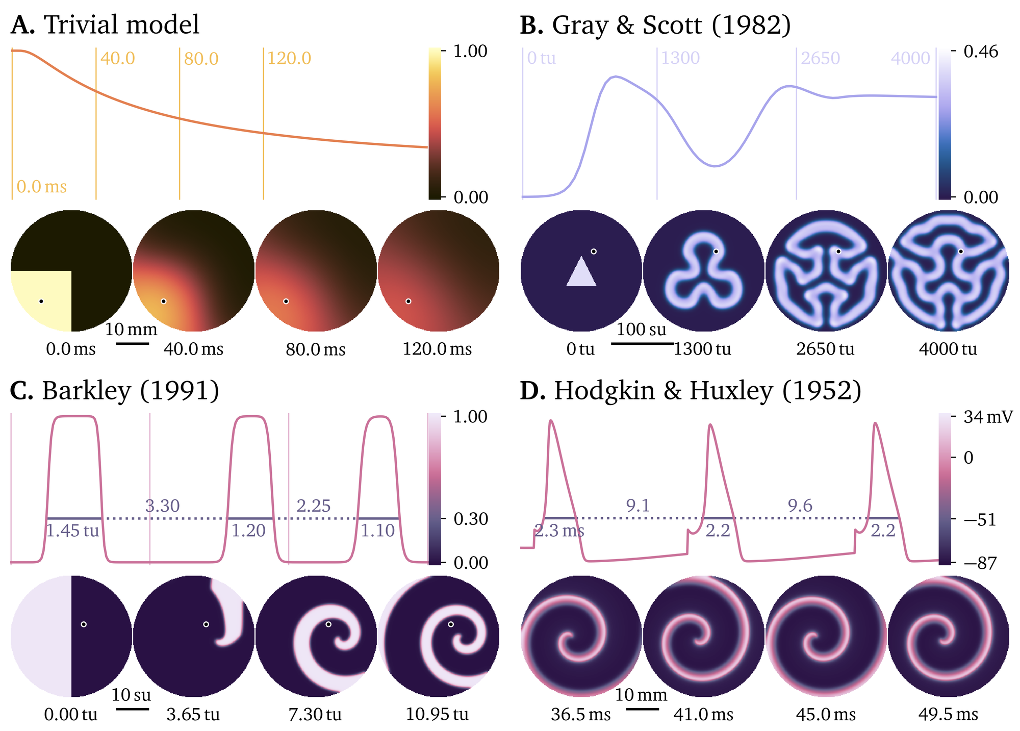
Figure 3: Pigreads includes various pre-defined models. The panels each contain a 2D simulation of a different model and a time trace at the marked reference point in the domain for manually chosen simulation parameters. See also the model overview in Table ¿tbl:models?. A. The trivial model defines diffusion of a single variable. B. The model by Gray & Scott (1983) describes the formation of various patterns depending on chosen parameters. C. One of the simplest models with excitation and recovery enabling spiral waves is the model by Barkley (1991). D. The model by Hodgkin & Huxley (1952) of the electrical conduction in giant nerve fibre of squids is one of the first mathematical models of electrophysiology. Here, instead of a time trace, we show a simulation of a single cell.
An overview of the pre-defined models for cardiac electrophysiology is
given in Fig. 4. The simulations shown in this figure
have been performed using resolutions, timings and stimuli that, for
each model, are found using an automatic procedure, as they depend on
the model’s dynamics: time step dt, grid spacing dx, and the
stimulus amplitude $\Delta u$ to be applied in a
region by instantaneously increasing the first variable by the given
value. In the remainder of this section, we outline this automatic
procedure to find these parameters for a given cardiac electrophysiology
model. Python scripts for this procedure are also published as a
separate, second repository.
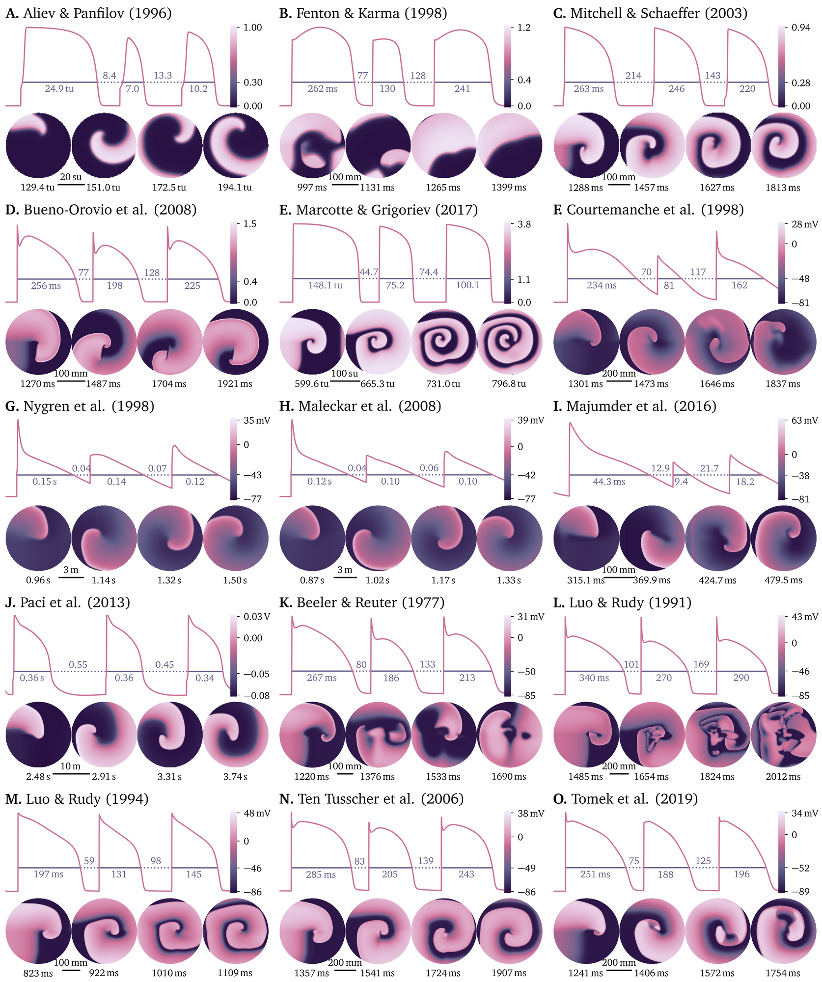
Figure 4: Models for cardiac electrophysiology that are pre-defined in Pigreads. For each model, we present a the transmembrane voltage for a simulation of a single cell of three pulses with different intervals between the pulses and a 2D simulation of a spiral wave initiated with an S0-S1-S2 protocol. See also the model overview in Table ¿tbl:models?. A.–E. Phenomenological models. F.–J. Models for atrial cells. K.–O. Models for ventricular cells. Note: The spiral wave is not necessarily stable in all models and may break up into spiral chaos.
First we must determine the time step
dtand the stimulus $\Delta u$. We consider a large space of possible values $(\mathtt{dt}, \Delta u) \in S \subset [{10}^{-8}, 0) \times [{10}^{-5}, {10}^{5}]$, in which we run single-cell simulations (${{\bm{{D}}}} = 0$). We then narrow down this search space $S$ to the valid regime $S' \subset S$ of a single action potential. We do so by checking these criteria:- Are all variables finite at all points in time?
- Does the first variable $u$ increase and decrease?
- Does $u$ oscillate less than five times?
- Does $u$ move away from the resting value?
- Does $u$ excite past the stimulated value?
- Does $u$ only change smoothly, i.e., without large jumps?
- Does $u$ cover a large fraction of the observed range of it across simulations?
We then pick
dtat the 80th percentile of valid simulations $S'$, followed by $\Delta u$ at the 30th percentile of valid simulations at the chosendt.We then run an additional single-cell simulation to determine the action potential duration (APD), i.e., the time that $u$ is above a 30% threshold.
With a 1D simulation at a very fine grid spacing
dxobtained via the CFL condition (Courant et al., 1928), we can then determine the conduction velocity (CV). Here, we for now set the diffusivity ${{\bm{{D}}}} = 1$ without loss of generality, as we can rescale it to any desired CV, as outlined below.We refine the values of CV and APD by measuring them for the third stimulus in 1D simulations with critical timings of stimulation.
In a series of 2D simulations at ${{\bm{{D}}}} = 1$, we determine the largest grid spacing
dxsuch that the difference between the fastest and slowest stimulation at some distance along the axes and diagonal to them is less than 5%.If necessary for numerical stability in 2D simulations, i.e., the CFL condition, we reduce
dt.
The result of this automatic procedure is given in a tabular overview of
all pre-defined models in Pigreads in Table ¿tbl:models?. This table
includes references to the original publications of the models with
their number of variables Nv, as well as the determined parameters for
discretisation, dt and dx, the stimulus strength
$\Delta u$, and resulting APD and CV at diffusivity
${{\bm{{D}}}} = 1$ in the units of the model. Note
that these parameters can be scaled to a desired velocity via:
$$
D \propto \mathrm{CV}^2,
\quad
\mathtt{dx} \propto \mathrm{CV},
\quad
\mathtt{dt} = \text{const}.
\qquad{(4)}$$ which follows for
Eq. 1 from keeping the velocity and diffusivity the same in
grid units, i.e.,
$D \cdot \mathtt{dt} / \mathtt{dx}^2$ and
$\mathrm{CV} \cdot \mathtt{dt}
/ \mathtt{dx}$ are both constant.
In cardiac electrophysiology, stimuli in the form of instantaneous changes in variables, like the provided $\Delta u$, are considered less physically realistic than current-based stimuli which take the form of a source term ${{\underline{{s}}}}$ in Eq. 1. Usually, a suitable amplitude of a current-based stimulus can be obtained by spreading out the stimulus $\Delta u$ over some time $T$: $$ s_0 = \frac{\Delta u}{T} \qquad{(5)}$$
While the provided stimulus amplitude $\Delta u$ and resolutions in time and space work well in our tests, they may not be optimal for all applications. The user may want to adjust them for their specific use case.
Positioning across alternatives
Most solvers for cardiac electrophysiology have no or only partial GPU support; these codes utilise parallelisation on large numbers of CPU cores, for instance alphabetically: Alya Red (Vázquez et al., 2016), BeatBox (Antonioletti et al., 2017), CEPS (Leguèbe et al., 2025), cbcbeat (E. Rognes et al., 2017), Chaste (Pitt-Francis et al., 2009), Continuity (Gonzales et al., 2016), fenicsx-beat (H. Finsberg, 2025), FiniteWave (Nezlobinsky et al., 2026), Ithildin (Kabus et al., 2024), lifex-ep (Africa et al., 2023), openCARP (Plank et al., 2021), OpenCMISS (Bradley et al., 2011), simcardems (H. N. T. Finsberg et al., 2023), and svMultiPhysics (Updegrove et al., 2016).
The solvers that use GPUs vary in terms of the numerical scheme, backend, and language used for the API to set up numerical simulations: Abubu.js is a finite-differences code using WebGL which is accessed via JavaScript in a web browser (Kaboudian et al., 2019); CardioMat uses finite differences in the Matlab Parallel Computing Toolbox (Biasi et al., 2025); and MonoAlg3D is a finite-volumes solver using MPI and CUDA that is interfaced with using custom INI files containing parameters (Berg et al., 2025).
Python’s robust packaging system, scientific libraries for numerical computing, data visualisation, and machine learning, as well as its ease of use, make it an attractive choice for developing scientific software. There is another GPU-based cardiac electrophysiology solver developed around the same time as Pigreads that also integrates well into the Python ecosystem: TorchCor uses finite elements with the PyTorch deep learning library (Zhou et al., 2026). Pigreads fundamentally differs from this as it uses finite differences and OpenCL as the backend. Due to the simpler numerical scheme and use of optimised low-level OpenCL code, Pigreads is usually faster than TorchCor for the same problem sizes. Pigreads solves the benchmark problem proposed by Niederer et al. (2011) around ten times faster than TorchCor: On the same hardware, TorchCor computes the solution in 9.2 s for the coarsest resolution, and 264 s for the finest resolution. For Pigreads’ performance, see section 3.
Outlook
While we here have focused on cardiac electrophysiology, Pigreads can be used for reaction-diffusion systems in general. Due to its simple API, it is easy to use and integrate into existing Python code, enabling researchers to build on a solid foundation. We envision that Pigreads will be used in the future for parameter estimation, inverse problems, uncertainty quantification, sensitivity analysis, and model reduction. It could also be integrated into clinical workflows for personalised medicine.
Its nature as a Python module also facilitates building, for instance, an interactive graphical user interface or a web application on top of it. This would make it even more accessible to a wider audience, for instance, to researchers without programming experience. We are including a proof-of-concept interactive demo in the Python module allowing to attempt to terminate atrial fibrillation, i.e., spiral chaos, by tapping a touch screen.
As new models can easily be defined, another use case is designing, fitting, and testing new models. The module could also be used for educational purposes, for instance in courses on mathematical biology, dynamical systems, or scientific computing.
While Pigreads could be extended in various ways – for instance more advanced time stepping methods, adaptive mesh refinement, support for more complex geometries, or other kinds of governing equations – we have chosen to keep the module minimal to keep it as stable as possible. While we are open to receive pull requests of minor tweaks, bugfixes, and additional model definitions and geometry files, no additional features should be added unless they are absolutely necessary. There is always the possibility to fork the project and add additional features if needed, for instance, on a per-project basis.
We hope that Pigreads will be a useful tool for researchers across various fields of science and that it will enable scientific progress.
Data availability
Pigreads can be installed from PyPI. The source code is available on GitLab, and its documentation on Read the Docs.
Scripts to generate the figures and data presented in this manuscript are available in a separate Git repository.
Addenda
Acknowledgments:
DK would like to thank Martina Chirilus-Bruckner and Daniël Pijnappels for inspiring discussions.
Declaration of generative AI and AI-assisted technologies in the manuscript preparation process. During the preparation of this work the authors used ChatGPT and GitHub Copilot in order to help with writing the manuscript and minor parts of the code. After using these tools, the authors reviewed and edited the content as needed and take full responsibility for the content of the published article.
Funding:
This work was supported by the Netherlands Organisation for Scientific Research (NWO Open Mind grant 2025/TTW/02025375 to TDC). DK was supported by KU Leuven grant GPUL/20/012, and the Society, Artificial Intelligence and Life Sciences (SAILS) initiative of Leiden University.
Competing interests:
The authors have declared that no competing interests exist.
Author contributions:
DK: Conceptualization, Methodology, Software, Validation, Formal analysis, Investigation, Resources, Data Curation, Writing – Original Draft, Writing – Review & Editing, Visualization. HD: Writing – Review & Editing, Supervision. TDC: Conceptualization, Writing – Review & Editing, Supervision, Project administration, Funding acquisition.
References
Africa, P. C., Piersanti, R., Regazzoni, F., Bucelli, M., Salvador, M., Fedele, M., Pagani, S., Dede’, L., & Quarteroni, A. (2023). lifex-ep: A robust and efficient software for cardiac electrophysiology simulations. BMC Bioinformatics, 24(1). https://doi.org/10.1186/s12859-023-05513-8
Antonioletti, M., Biktashev, V. N., Jackson, A., Kharche, S. R., Stary, T., & Biktasheva, I. V. (2017). BeatBox–HPC simulation environment for biophysically and anatomically realistic cardiac electrophysiology. PLOS ONE, 12(5), e0172292. https://doi.org/10.1371/journal.pone.0172292
Barkley, D. (1991). A model for fast computer simulation of waves in excitable media. Physica D: Nonlinear Phenomena, 49(1–2), 61–70. https://doi.org/10.1016/0167-2789(91)90194-e
Berg, L. A., Oliveira, R. S., Camps, J., Wang, Z. J., Doste, R., Bueno-Orovio, A., Santos, R. W. dos, & Rodriguez, B. (2025). MonoAlg3D: Enabling cardiac electrophysiology digital twins with an efficient open source scalable solver on GPU clusters. https://doi.org/10.1101/2025.04.09.647733
Biasi, N., Seghetti, P., Parollo, M., Zucchelli, G., & Tognetti, A. (2025). A Matlab toolbox for cardiac electrophysiology simulations on patient-specific geometries. Computers in Biology and Medicine, 185, 109529. https://doi.org/10.1016/j.compbiomed.2024.109529
Bradley, C., Bowery, A., Britten, R., Budelmann, V., Camara, O., Christie, R., Cookson, A., Frangi, A. F., Gamage, T. B., Heidlauf, T., Krittian, S., Ladd, D., Little, C., Mithraratne, K., Nash, M., Nickerson, D., Nielsen, P., Nordbø, Ø., Omholt, S., Pashaei, A., Paterson, D., Rajagopal, V., Reeve, A., Röhrle, O., Safaei, S., Sebastián, R., Steghöfer, M., Wu, T., Yu, T., Zhang, H., & Hunter, P. (2011). OpenCMISS: A multi-physics & multi-scale computational infrastructure for the VPH/Physiome project. Progress in Biophysics and Molecular Biology, 107(1), 32–47. https://doi.org/10.1016/j.pbiomolbio.2011.06.015
Cannon, J., McCarthy, M. M., Lee, S., Lee, J., Börgers, C., Whittington, M. A., & Kopell, N. (2014). Neurosystems: Brain rhythms and cognitive processing. European Journal of Neuroscience, 39(5), 705–719. https://doi.org/10.1111/ejn.12453
Clayton, R., Bernus, O., Cherry, E. M., Dierckx, H., Fenton, F. H., Mirabella, L., Panfilov, A. V., Sachse, F. B., Seemann, G., & Zhang, H. (2011). Models of cardiac tissue electrophysiology: Progress, challenges and open questions. Progress in Biophysics and Molecular Biology, 104(1-3), 22–48. https://doi.org/10.1016/j.pbiomolbio.2010.05.008
Clerx, M., Collins, P., De Lange, E., & Volders, P. G. (2016). Myokit: A simple interface to cardiac cellular electrophysiology. Progress in Biophysics and Molecular Biology, 120(1-3), 100–114. https://doi.org/10.1016/j.pbiomolbio.2015.12.008
Clerx, M., Cooling, M. T., Cooper, J., Garny, A., Moyle, K., Nickerson, D. P., Nielsen, P. M., & Sorby, H. (2020). CellML 2.0. Journal of Integrative Bioinformatics, 17(2-3), 20200021. https://doi.org/10.1515/jib-2020-0021
Courant, R., Friedrichs, K., & Lewy, H. (1928). Über die partiellen Differenzengleichungen der mathematischen Physik. Mathematische Annalen, 100(1), 32–74. https://doi.org/10.1007/BF01448839
Courtemanche, M., Ramirez, R. J., & Nattel, S. (1998). Ionic mechanisms underlying human atrial action potential properties: Insights from a mathematical model. American Journal of Physiology-Heart and Circulatory Physiology, 275(1), H301–H321. https://doi.org/10.1152/ajpheart.1998.275.1.h301
De Coster, T., Claus, P., Seemann, G., Willems, R., Sipido, K. R., & Panfilov, A. V. (2018). Myocyte remodeling due to fibro-fatty infiltrations influences arrhythmogenicity. Frontiers in Physiology, 9. https://doi.org/10.3389/fphys.2018.01381
Dossel, O., Krueger, M. W., Weber, F. M., Schilling, C., Schulze, W. H. W., & Seemann, G. (2011). A framework for personalization of computational models of the human atria. 2011 Annual International Conference of the IEEE Engineering in Medicine and Biology Society, 4324–4328. https://doi.org/10.1109/iembs.2011.6091073
E. Rognes, M., E. Farrell, P., W. Funke, S., E. Hake, J., & M. C. Maleckar, M. (2017). cbcbeat: An adjoint-enabled framework for computational cardiac electrophysiology. The Journal of Open Source Software, 2(13), 224. https://doi.org/10.21105/joss.00224
Finsberg, H. (2025). fenicsx-beat - an open source simulation framework for cardiac electrophysiology. Journal of Open Source Software, 10(114), 8416. https://doi.org/10.21105/joss.08416
Finsberg, H. N. T., Herck, I. G. M. van, Daversin-Catty, C., Arevalo, H., & Wall, S. (2023). simcardems: A FEniCS-based cardiac electro-mechanics solver. Journal of Open Source Software, 8(81), 4753. https://doi.org/10.21105/joss.04753
FitzHugh, R. (1961). Impulses and physiological states in theoretical models of nerve membrane. Biophysical Journal, 1(6), 445–466. https://doi.org/10.1016/s0006-3495(61)86902-6
Gonzales, M., Guthals, A., Kerckhoffs, R., Krishnamurthy, A., Lionetti, F., Van Dorn, J., Villongco, C., Vincent, K., & McCulloch, A. (2016). Continuity: A problem-solving environment for multiscale biological modeling [Computer software]. Cardiac Mechanics Research Group; University of California, San Diego. https://continuity.ucsd.edu
Gray, P., & Scott, S. K. (1983). Autocatalytic reactions in the isothermal, continuous stirred tank reactor. Chemical Engineering Science, 38(1), 29–43. https://doi.org/10.1016/0009-2509(83)80132-8
Harris, C. R., Millman, K. J., Walt, S. J. van der, Gommers, R., Virtanen, P., Cournapeau, D., Wieser, E., Taylor, J., Berg, S., Smith, N. J., Kern, R., Picus, M., Hoyer, S., Kerkwijk, M. H. van, Brett, M., Haldane, A., Río, J. F. del, Wiebe, M., Peterson, P., Gérard-Marchant, P., Sheppard, K., Reddy, T., Weckesser, W., Abbasi, H., Gohlke, C., & Oliphant, T. E. (2020). Array programming with NumPy. Nature, 585(7825), 357–362. https://doi.org/10.1038/s41586-020-2649-2
Hodgkin, A. L., & Huxley, A. F. (1952). A quantitative description of membrane current and its application to conduction and excitation in nerve. The Journal of Physiology, 117(4), 500–544. https://doi.org/10.1113/jphysiol.1952.sp004764
Hren, R. (1996). A realistic model of the human ventricular myocardium: Application to the study of ectopic activation. [PhD thesis, Dalhousie University]. https://dalspace.library.dal.ca//handle/10222/55139
Hren, R. (1998). Value of epicardial potential maps in localizing pre-excitation sites for radiofrequency ablation. A simulation study. Physics in Medicine and Biology, 43(6), 1449–1468. https://doi.org/10.1088/0031-9155/43/6/006
Hunter, J. D. (2007). Matplotlib: A 2D graphics environment. Computing in Science & Engineering, 9(3), 90–95. https://doi.org/10.1109/MCSE.2007.55
Kaboudian, A., Cherry, E. M., & Fenton, F. H. (2019). Real-time interactive simulations of large-scale systems on personal computers and cell phones: Toward patient-specific heart modeling and other applications. Science Advances, 5(3). https://doi.org/10.1126/sciadv.aav6019
Kabus, D., Cloet, M., Zemlin, C., Bernus, O., & Dierckx, H. (2024). The Ithildin library for efficient numerical solution of anisotropic reaction-diffusion problems in excitable media. PLOS ONE, 19(9), 1–26. https://doi.org/10.1371/journal.pone.0303674
Kapral, R., & Showalter, R. (1995). Chemical waves and patterns. Kluwer.
Keldermann, R. H., ten Tusscher, K. H. W. J., Nash, M. P., Bradley, C. P., Hren, R., Taggart, P., & Panfilov, A. V. (2009). A computational study of mother rotor VF in the human ventricles. American Journal of Physiology-Heart and Circulatory Physiology, 296(2), H370–H379. https://doi.org/10.1152/ajpheart.00952.2008
Klöckner, A., Pinto, N., Lee, Y., Catanzaro, B., Ivanov, P., & Fasih, A. (2012). PyCUDA and PyOpenCL: A scripting-based approach to GPU run-time code generation. Parallel Computing, 38(3), 157–174. https://doi.org/10.1016/j.parco.2011.09.001
Lechleiter, J., Girard, S., Peralta, E., & Clapham, D. (1991). Spiral calcium wave propagation and annihilation in xenopus laevis oocytes. Science, 252(5002), 123–126. https://doi.org/10.1126/science.2011747
Leguèbe, M., Coudière, Y., Calvez, L., Pannetier, V., Douanla-Lontsi, C., Davidović, A., Bécue, P.-E., Juhoor, M., & Zemzemi, N. (2025). CEPS: A cardiac electrophysiology exploration tool for new mathematical models and methods. Journal of Open Source Software, 10(114), 8910. https://doi.org/10.21105/joss.08910
Marcotte, C. D., & Grigoriev, R. O. (2017). Dynamical mechanism of atrial fibrillation: A topological approach. Chaos: An Interdisciplinary Journal of Nonlinear Science, 27(9). https://doi.org/10.1063/1.5003259
Murray, J. (1976). On travelling wave solutions in a model for the belousov-zhabotinskii reaction. Journal of Theoretical Biology, 56(2), 329–353. https://doi.org/10.1016/S0022-5193(76)80078-1
Nagumo, J., Arimoto, S., & Yoshizawa, S. (1962). An active pulse transmission line simulating nerve axon. Proceedings of the IRE, 50(10), 2061–2070. https://doi.org/10.1109/jrproc.1962.288235
Net, T. A. A. döt, Ingy AND Müller. (2023). YAML ain’t markup language, revision 1.2.2. YAML Language Development Team. https://yaml.org/spec/1.2.2/
Nezlobinsky, T., Okenov, A., Vandersickel, N., & Panfilov, A. V. (2026). Finitewave: A lightweight and accessible framework for cardiac electrophysiology simulations [Computer software]. Ghent University, Belgium. https://github.com/finitewave/Finitewave
Niederer, S. A., Kerfoot, E., Benson, A. P., Bernabeu, M. O., Bernus, O., Bradley, C., Cherry, E. M., Clayton, R., Fenton, F. H., Garny, A., Heidenreich, E., Land, S., Maleckar, M., Pathmanathan, P., Plank, G., Rodríguez, J. F., Roy, I., Sachse, F. B., Seemann, G., Skavhaug, O., & Smith, N. P. (2011). Verification of cardiac tissue electrophysiology simulators using an N-version benchmark. Philosophical Transactions of the Royal Society A: Mathematical, Physical and Engineering Sciences, 369(1954), 4331–4351. https://doi.org/10.1098/rsta.2011.0139
Pitt-Francis, J., Pathmanathan, P., Bernabeu, M. O., Bordas, R., Cooper, J., Fletcher, A. G., Mirams, G. R., Murray, P., Osborne, J. M., Walter, A., Chapman, S. J., Garny, A., Leeuwen, I. M. M. van, Maini, P. K., Rodríguez, B., Waters, S. L., Whiteley, J. P., Byrne, H. M., & Gavaghan, D. J. (2009). Chaste: A test-driven approach to software development for biological modelling. Computer Physics Communications, 180(12), 2452–2471. https://doi.org/10.1016/j.cpc.2009.07.019
Plank, G., Loewe, A., Neic, A., Augustin, C., Huang, Y.-L., Gsell, M. A. F., Karabelas, E., Nothstein, M., Prassl, A. J., Sánchez, J., Seemann, G., & Vigmond, E. J. (2021). The openCARP simulation environment for cardiac electrophysiology. Computer Methods and Programs in Biomedicine, 208, 106223. https://doi.org/10.1016/j.cmpb.2021.106223
Rotermund, H.-H., Engel, W., Kordesch, M., & Ertl, G. (1990). Imaging of spatio-temporal pattern evolution during carbon monoxide oxidation on platinum. Nature, 343(6256), 355–357. https://doi.org/10.1038/343355a0
Stone, J. E., Gohara, D., & Shi, G. (2010). OpenCL: A parallel programming standard for heterogeneous computing systems. Computing in Science & Engineering, 12(3), 66–73. https://doi.org/10.1109/MCSE.2010.69
Sullivan, B., & Kaszynski, A. (2019). PyVista: 3D plotting and mesh analysis through a streamlined interface for the Visualization Toolkit (VTK). Journal of Open Source Software, 4(37), 1450. https://doi.org/10.21105/joss.01450
ten Tusscher, K. H. W. J., & Panfilov, A. V. (2006). Alternans and spiral breakup in a human ventricular tissue model. American Journal of Physiology-Heart and Circulatory Physiology, 291(3), H1088–H1100. https://doi.org/10.1152/ajpheart.00109.2006
Updegrove, A., Wilson, N. M., Merkow, J., Lan, H., Marsden, A. L., & Shadden, S. C. (2016). SimVascular: An open source pipeline for cardiovascular simulation. Annals of Biomedical Engineering, 45(3), 525–541. https://doi.org/10.1007/s10439-016-1762-8
van Rossum, G., Drake, F. L., et al. (1995). The Python programming language. Centrum voor Wiskunde en Informatica Amsterdam. https://www.python.org
Vázquez, M., Houzeaux, G., Koric, S., Artigues, A., Aguado-Sierra, J., Arís, R., Mira, D., Calmet, H., Cucchietti, F., Owen, H., Taha, A., Burness, E. D., Cela, J. M., & Valero, M. (2016). Alya: Multiphysics engineering simulation toward exascale. Journal of Computational Science, 14, 15–27. https://doi.org/10.1016/j.jocs.2015.12.007
Zhou, B., Balmus, M., Corrado, C., Cicci, L., Qian, S., & Niederer, S. A. (2026). TorchCor: High-performance cardiac electrophysiology simulations with the finite element method on GPUs. SoftwareX, 33, 102521. https://doi.org/10.1016/j.softx.2027.102521