
This article was previously published in PLOS ONE 19(9): e0303674 (Kabus, Cloet, et al., 2024) and is a chapter of my dissertation.
Authors:
Desmond Kabus1,2 (ORCID: 0000-0002-6965-5211)
Marie Cloet1 (ORCID: 0000-0002-8974-6401)
Christian Zemlin3 (ORCID: 0000-0001-5834-5544)
Olivier Bernus4 (ORCID: 0000-0003-3917-5791)
Hans Dierckx1 (ORCID: 0000-0003-0899-8082)
Institutions:
Department of Mathematics, KU Leuven Campus Kortrijk (KULAK), Etienne Sabbelaan 53, 8500 Kortrijk, Belgium
Laboratory of Experimental Cardiology, Leiden University Medical Center (LUMC), Albinusdreef 2, 2333 ZA Leiden, The Netherlands
Division of Cardiothoracic Surgery, Department of Surgery, University of Washington School of Medicine, 660 South Euclid Avenue, 63110 St Louis, MO, United States of America
Univ. Bordeaux, Inserm, Centre de Recherche Cardio-Thoracique de Bordeaux U1045, IHU Liryc, Hôpital Xavier Arnozan, Avenue du Haut Lévêque, 33600 Pessac, France
Correspondence: [email protected]
DOI: 10.1371/journal.pone.0303674
Editor: Rafael Sachetto Oliveira, Universidade Federal de Sao Joao del-Rei, Brazil
Keywords:
- excitable media
- cardiac electrophysiology
- open-source
- finite differences
- anisotropic diffusion
- reaction-diffusion equation
- C++
Abstract:
Ithildin is an open-source library and framework for efficient parallelized simulations of excitable media, written in the C++ programming language. It uses parallelization on multiple CPU processors via the message passing interface (MPI). We demonstrate the library’s versatility through a series of simulations in the context of the monodomain description of cardiac electrophysiology, including the S1S2 protocol, spiral break-up, and spiral waves in ventricular geometry. Our work demonstrates the power of Ithildin as a tool for studying complex wave patterns in cardiac tissue and its potential to inform future experimental and theoretical studies. We publish our full code with this paper in the name of open science.
Popular summary:
We present Ithildin, an open-source library for reaction-diffusion systems such as the electrical waves in cardiac tissue controlling the heart beat. We demonstrate the versatility of Ithildin by example simulations in various cell models and geometries, from simple 2D simulations to detailed ones in ventricular geometry. Our simulations highlight key features of Ithildin, such as recording pseudo-electrograms or filament trajectories. We hope that our work will contribute to the growing understanding of cardiac electrophysiology and inform future experimental and theoretical studies.
Introduction
With the Ithildin framework, we want to open up new gateways in the numerical simulation of reaction-diffusion systems, such as the electrical activation patterns in the heart.1
Our motivation to write a reaction-diffusion solver comes from the numerical study of electrical patterns inside the heart (Clayton et al., 2011). These patterns, which are incompletely understood, are a main cause of death and even as a chronic disease, they complicate people’s lives. In the past decades, computer models of arrhythmia have allowed mechanistic insight in the origin and control of arrhythmias (Fenton & Karma, 1998). On the longer term, it is thought that digitized versions of patients' hearts could help offer better diagnostics and planning of procedures; such personalized heart models are called cardiac digital twins (Gillette et al., 2021; Koopsen et al., 2024; Niederer et al., 2019; Trayanova et al., 2020). In view of open science, we have decided to share the code that has been steadily developed in our group since 2007 with the scientific community.
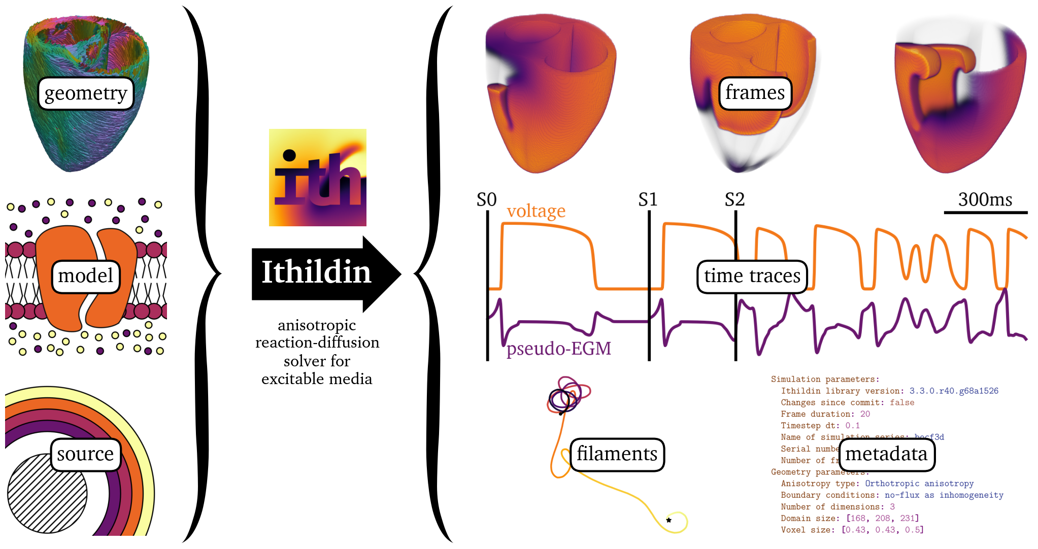
Figure 1: Ithildin can be used to solve reaction-diffusion problems in excitable media. Required inputs for the software are: the diffusion tensor and geometry of a medium—such as the heart muscle, a reaction term—the so-called model, and source terms—typically a stimulation protocol. Ithildin can then calculate the evolution of the model variables in the medium over time. During calculation, Ithildin records relevant spatio-temporal data and metadata, as well as detecting rotor cores as filaments. The data visualized here are taken from several simulations which will be discussed below.
A flowchart outlining the functionality of Ithildin can be found in Fig. 1. Ithildin is designed to comply with the 2011 version of the ISO-C++ standard (ISO, 2011), but it compiles with all newer versions, including the current 2023 ISO-C++ standard (ISO, 2014, 2017, 2020, 2023). The software facilitates forward Euler and Runge-Kutta finite-difference solutions for reaction-diffusion systems in $N$-dimensional space, such as the monodomain equation for cardiac electrophysiology, with specified boundary conditions (Clayton et al., 2011).
The framework offers quick computation through CPU parallelization using OpenMPI (Graham et al., 2006). It also boasts decent documentation of available features, made accessible through Doxygen (van Heesch, 2023). Ithildin writes easy-to-parse YAML log files to document simulation setups (döt Net et al., 2023). Additionally, it allows convenient output of frames of recorded variables at regular intervals in the form of NumPy NPY files (Harris et al., 2020). The software supports easy and powerful post-processing with the Python module for Ithildin (Kabus et al., 2022), including integration with Scientific Python (Virtanen et al., 2020), 2D visualization with Matplotlib (Hunter, 2007), and 3D visualization with ParaView (Ahrens et al., 2005).
Ithildin also allows the recording of pseudo-electrograms (EGMs) and state variables at full numerical time resolution, as well as the tracking of filaments, which represent the instantaneous rotation axes of rotors. The software features a flexible setup for in-silico experiments, also called simulations, through a simple class-based C++ interface.
Various types of geometries are implemented, ranging from a simple 1D
cable and spirals in 2D tissue to whole-heart geometry and even 4D
hyperspace. The space can be partitioned to use multiple cell models in
the same experiment via Model_multi. Realistic stimulation protocols
can be added as Stimulus objects and may be started by a Trigger.
Ithildin also includes a logging system with minimal impact on
computation speed and various levels of verbosity.
In this paper, we provide an overview of this framework, guiding the reader through its components. Results from several in-silico experiments are presented as the main components of Ithildin are introduced. The details of these so-called simulations are outlined towards the end of this paper in section 5, along with a tabular overview in Table 4.
Essential numerical methods
Reaction-diffusion system
The diffusion of electrical signals in cardiac tissue can be modelled as a reaction-diffusion system, where the diffusion tensor ${{\bm{{D}}}}$ represents the anisotropic properties of the medium. This tensor encapsulates the spatial orientation of fibers in the medium and the effects of inhomogeneities on signal propagation. With the local unit vectors along the fibers ${{\bm{{e}}}}_{\text{f}}$, normal to fibers in the sheet plane ${{\bm{{e}}}}_{\text{s}}$, and normal to both of these ${{\bm{{e}}}}_{\!\times\!} = {{\bm{{e}}}}_{\text{f}} \times {{\bm{{e}}}}_{\text{s}}$, forming a orthonormal basis, the fiber orientation is encoded using diffusivities $D_{{\text{f}}, {\text{s}}, {\!\times\!}}{{\left( {{\bm{{x}}}} \right)}}$ in each of these directions (Clayton et al., 2011): $$ {{\bm{{D}}}} = D_{\text{f}} {{\bm{{e}}}}_{\text{f}} {{{{\bm{{e}}}}_{\text{f}}}^\mathrm{T}} + D_{\text{s}} {{\bm{{e}}}}_{\text{s}} {{{{\bm{{e}}}}_{\text{s}}}^\mathrm{T}} + D_{\!\times\!} {{\bm{{e}}}}_{\!\times\!} {{{{\bm{{e}}}}_{\!\times\!}}^\mathrm{T}} \qquad{(1)}$$
The core equation governing the evolution of the state variable vector ${{\underline{{u}}}}$ is the reaction-diffusion equation: $$ \partial_t {{\underline{{u}}}} = {{\underline{{P}}}} \nabla \cdot {{\bm{{D}}}} \nabla {{\underline{{u}}}} + {{\underline{{r}}}}{{\left( {{\underline{{u}}}} \right)}} \qquad{(2)}$$ or in index notation: $$ \partial_t u_m{{\left( t,{{\bm{{x}}}} \right)}} = \textstyle\sum_{m'} P_{mm'} \; \textstyle\sum_{n} \partial_{n} \textstyle\sum_{n'} D_{nn'}{{\left( {{\bm{{x}}}} \right)}} \; \partial_{n'} u_{m'}{{\left( t, {{\bm{{x}}}} \right)}} + r_{m}{{\left( {{\underline{{u}}}};{{\bm{{x}}}} \right)}} \qquad{(3)}$$ for $m, m' \in {{\left\{1,...,M \right\}}}$ with the number of state variables $M$, and $n, n' \in {{\left\{1,...,N \right\}}}$ with the number of spatial dimensions $N$, using the notation $\partial_n = \partial_{x_n}$ for the spatial partial derivatives.
Here, ${{\underline{{u}}}}$ is the state variable vector and ${{\underline{{r}}}}({{\underline{{u}}}})$ accounts for the reaction term and is called the model. We refer to the first component of ${{\underline{{u}}}}$ as $u$, which for electrophysiological models is the transmembrane voltage $V_\text{m}$ or a rescaled version of it, see also section 4.2. For two-variable models, the second component of ${{\underline{{u}}}}$ is often referred to as the restitution or recovery variable $v$. In the term representing diffusion, ${{\bm{{D}}}}$ is determined by the geometry of the medium and the presence of inhomogeneities, see section 4.1. The projection matrix ${{\underline{{P}}}}$ is typically a diagonal matrix describing whether or not a variable is diffused. For instance, only the first variable of the AP96 model (Aliev & Panfilov, 1996) is diffused, such that ${{\underline{{P}}}} = {\operatorname{diag}{{\left( 1, 0 \right)}}}$.
Different notation is used to distinguish between vectors ${{\bm{{x}}}}$ and matrices ${{\bm{{D}}}}$ in physical space in bold font, and underlined vectors ${{\underline{{u}}}}$ and matrices ${{\underline{{P}}}}$ with respect to state variables. We use lowercase letters for vectors and uppercase for matrices. An overview of the most relevant quantities in Ithildin is given in Table 1.
| symbol | dimension | unit | name |
|---|---|---|---|
| $N$ | $\in\mathbb N$ | 1 | number of spatial dimensions |
| $M$ | $\in\mathbb N$ | 1 | number of state variables |
| $t$ | $\in \mathbb R_+$ | ms | time |
| ${{\bm{{x}}}}$ | $\in \Omega \subset \mathbb R^N$ | mm | space |
| ${{\underline{{u}}}}{{\left( t, {{\bm{{x}}}} \right)}}$ | $\in \mathbb R^M$ | $\star$ (various units) | state variables |
| ${{\underline{{r}}}}{{\left( {{\bm{{x}}}}, {{\underline{{u}}}} \right)}}$ | $\in \mathbb R^M$ | $\star$/ms | reaction term, model function |
| ${{\bm{{D}}}}{{\left( {{\bm{{x}}}} \right)}}$ | $\in \mathbb R^{N\times N}$ | mm²/ms | diffusion tensor |
| ${{\underline{{P}}}}$ | $\in \mathbb R^{M\times M}$ | 1 | projection matrix |
Table 1: Quantities in the reaction-diffusion problem.
Ithildin obtains approximate solutions of the reaction-diffusion equation (Eq. 2) via a finite-differences approach: Time $t$ and space ${{\bm{{x}}}}$ are discretized on a grid and values ${{\underline{{u}}}}{{\left( t, {{\bm{{x}}}} \right)}}$ are associated with the vertices of this grid. We choose a fixed temporal resolution, the time step $\Delta t$, and constant spatial grid spacing $\Delta {{\bm{{x}}}}$. The values ${{\underline{{u}}}}{{\left( t + \Delta t, {{\bm{{x}}}} \right)}}$ at a subsequent time-step are computed based on the previous ones, according to discretized versions of the governing equations, i.e., the reaction-diffusion equation (Eq. 2), together with boundary and initial conditions.
Time integration
Starting from an initial state, the state variable vector ${{\underline{{u}}}}$ is integrated over time using a so-called time stepping scheme leading to an approximate solution of the reaction-diffusion system using finite differences. Ithildin implements two main stepping schemes to choose from: forward Euler and the classic Runge-Kutta method (RK4) (Euler, 1794; Press, 2007).
Defining ${{\underline{{f}}}}$ as the right hand side of the reaction-diffusion equation (Eq. 2), the forward Euler method takes the form (Press, 2007): $$ {{\underline{{u}}}} {{\left( t + \Delta t, {{\bm{{x}}}} \right)}} = {{\underline{{u}}}} {{\left( t, {{\bm{{x}}}} \right)}} + \Delta t \, {{\underline{{f}}}} {{\left( t, {{\bm{{x}}}}; {{\underline{{u}}}} \right)}} + O{{\left( \Delta t^2 \right)}} \qquad{(4)}$$ This method is the default time integration scheme in Ithildin. Despite its numerical error being of order $O{{\left( \Delta t^2 \right)}}$, with a sufficiently small time step, the accuracy of the Euler method is adequate for our use cases.
Due to the Courant-Friedrichs-Lewy condition (CFL), a stability
criterion for the integration of the reaction-diffusion equation,
$\Delta t$ needs to be chosen sufficiently small
(Courant et al., 1928). Ithildin automatically
chooses an appropriate time step based on the CFL condition for the
different supported geometries,
cf. section 4.1. For example, for the
most simple implemented geometry contained in Ithildin, i.e., isotropic
diffusion (see Geometry_Iso in
section 4.1 and
Table 2), the CFL condition is enforced by
setting (Li et al., 1994):
$$
\Delta t
<
{{\left[ 2\max{{{\underline{{P}}}}} \sum_{n=1}^{N} \frac{D_{nn}}{\Delta x_n^2} \right]}}^{-1}
\qquad{(5)}$$ where
$D_{nn}$ are the diagonal components of
${{\bm{{D}}}}$ and
$\max{{{\underline{{P}}}}}$ is the maximum value of
${{\underline{{P}}}}$.
Higher accuracy at the cost of more computations per time step, can be achieved with the RK4 method (Press, 2007): $$\begin{aligned} {{\underline{{u}}}} {{\left( t + \Delta t, {{\bm{{x}}}} \right)}} &= {{\underline{{u}}}} {{\left( t, {{\bm{{x}}}} \right)}} + \frac{1}{6}\Delta{{\underline{{u}}}}_1 + \frac{1}{3}\Delta{{\underline{{u}}}}_2 + \frac{1}{3}\Delta{{\underline{{u}}}}_3 + \frac{1}{6}\Delta{{\underline{{u}}}}_4 + O{{\left( \Delta t^5 \right)}} \\ \Delta{{\underline{{u}}}}_1 &:= \Delta t\, {{\underline{{f}}}} {{\left( t, {{\bm{{x}}}}; {{\underline{{u}}}} \right)}} \\ \Delta{{\underline{{u}}}}_2 &:= \Delta t\, {{\underline{{f}}}} {{\left( t + \textstyle\frac{1}{2}\Delta t, {{\bm{{x}}}}; {{\underline{{u}}}} + \textstyle\frac{1}{2}\Delta{{\underline{{u}}}}_1 \right)}} \\ \Delta{{\underline{{u}}}}_3 &:= \Delta t\, {{\underline{{f}}}} {{\left( t + \textstyle\frac{1}{2}\Delta t, {{\bm{{x}}}}; {{\underline{{u}}}} + \textstyle\frac{1}{2}\Delta{{\underline{{u}}}}_2 \right)}} \\ \Delta{{\underline{{u}}}}_4 &:= \Delta t\, {{\underline{{f}}}} {{\left( t + \Delta t, {{\bm{{x}}}}; {{\underline{{u}}}} + \Delta{{\underline{{u}}}}_3 \right)}} \end{aligned}\qquad{(6)}$$ Note that ${{\underline{{f}}}}$ needs to be evaluated four times for the RK4 method and only once for the Euler method. While RK4 is still an explicit method subject to instability at too large $\Delta t$, a larger $\Delta t$ value than for the Euler method can typically be used.
The stepping scheme to be used can be chosen in Ithildin on a
per-variable level via Model::steppings.
Numerical spatial derivatives
For the numerical solution of the reaction-diffusion equation (Eq. 2), the spatial derivative in its right hand side must be computed, i.e., the diffusion operator ${{\underline{{P}}}}\nabla\cdot{{\bm{{D}}}}\nabla{{\underline{{u}}}}$. This is implemented as weighted sums of the value of ${{\underline{{u}}}}$ at neighboring vertices on the grid of the discretized domain. The weights for the calculation of the stencil depend on the chosen type of diffusion (section 4.1). The two main types in this software are a first order stencil, including only the nearest neighbors, and a second order stencil, including also the next to nearest neighbors.
In the simplest case (see Geometry_Iso in
section 4.1 and
Table 2), we consider isotropic and
homogeneous diffusivity. The diffusion operator can then be computed via
the Laplacian operator $\nabla^2$. This is done with
a 5-point stencil for the 2D case, a 7-point stencil for the 3D case,
etc., see also Fig. 2, panel (a). Consequently,
the weights are calculated as: $$
\begin{aligned}
w_n &= \frac{1}{\Delta x_n} \quad \text{for }1\leq n\leq 2 N
\\
w_0 &= -\sum_{n=1}^{2N}w_n
\end{aligned}
\qquad{(7)}$$ where
$N$ is the number of dimensions and
$\Delta x_n$ is the grid resolution in the direction
of the neighbor corresponding to weight $w_i$, e.g.,
$\Delta x_5 = \Delta z$. Note that the indices
correspond to those displayed in Fig. 2.
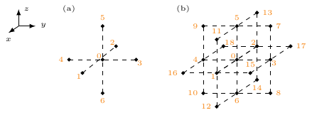
Figure 2: Stencils for isotropic diffusion (a) and orthotropic diffusion (b) with numbering of the involved grid points.
For the more general orthotropic diffusion, the stencil for numerical
differentiation includes the nearest and diagonal neighbors of a grid
point, see Fig. 2, panel (b). The weights for
orthotropic diffusion are obtained by a combination of central
differences approximations to derivatives and linear interpolation of
values between two grid points. For more details, the reader is referred
to the documentation of Geometry_OrtAniso.
Implementation
The source code of Ithildin is written in the C++ programming language, following the 2011 version of the ISO-C++ standard (ISO, 2011). This was chosen to facilitate programming at a level relatively close to the hardware, but also using some of the useful data-structures that are contained in the standard template library (STL).
Ithildin is designed to run in parallel on multiple CPU cores using MPI,
specifically OpenMPI (Graham et al., 2006). Using the
mpirun command, multiple instances, also known as processes, of the
same compiled executable are started that run across different processor
cores. The processes are then coordinated such that there is one
so-called manager process, that manages a bunch of so-called worker
processes. The manager does an equal share of the computational work,
just like a worker. The only difference is that the manager distributes
and directs information to be exchanged from one process to another. In
Ithildin, the memory is not shared across processes, instead each
process works on its share of the computational domain. We split the
domain in the $x$-direction, such that each process
is responsible for computations on a roughly equal share of vertices
inside the to-be-simulated medium. Even when some parts of the domain
are classified as exterior points, i.e., points on which no calculations
need to be performed, they are taken into account when splitting the
domain between processes. This splitting is possible because the
reaction-diffusion systems to be studied with Ithildin are local,
meaning that the temporal evolution at each time $t$
and each point ${{\bm{{x}}}}$ in space depends only
on the current state vector
${{\underline{{u}}}}{{\left( t, {{\bm{{x}}}} \right)}}$
at that position and its spatial derivatives
(Eq. 2). Internally, a layer of so-called ghost
points is added around each process’ part of the domain such that the
spatial derivatives can still be calculated in the same way as for any
other point in the domain
(section 2.3). The values
${{\underline{{u}}}}$ on these ghost points are
exchanged with the neighboring processes, as coordinated by the manager
process. Additional ghost points are also used to enforce Neumann
boundary conditions, which is done by setting the weights for the
calculation of the numerical spatial derivatives accordingly.
To run a simulation in Ithildin, the user needs to define a main()
function that is to be called by all subprocesses. This is usually done
using a C++ file calling the required components of the Ithildin library
defining the main() function, a so-called main file. Ithildin can be
installed as a shared library on Unix-based systems that is required by
executables obtained from compiling main files. Alternatively, it is
also possible to statically compile the Ithildin library with a main
file into a stand-alone executable.
Besides the necessary preparations for using MPI, running a simulation
using Ithildin’s Sim class requires three main components, which are
instances of three classes:
Model: the reaction term ${{\underline{{r}}}}{{\left( {{\underline{{u}}}} \right)}}$, typically a cell model,Geometry: the discretized diffusion term ${{\underline{{P}}}} \nabla \cdot {{\bm{{D}}}} \nabla {{\underline{{u}}}}$ for a chosen geometry of the medium, andSource: the stimulus protocol to use as well as inhomogeneities in the medium.
In the following section 4, an overview is given for each of these classes and their derived classes. Combining all of the components, an illustrative, minimal main file can be obtained, in which a planar wave crosses the medium in positive $x$-direction:
#include "ithildin.h"

int main(int argc, char** argv){
    // 0. initialize MPI
    Mpiclass mpi(argc, argv);

    // 1. select reaction term
    Model_SmooKa model;

    // 2. select diffusion term
    vector<int> size{30, 30, 1};
    vector<float> dx{1., 1., 1.};
    Geometry_Iso geom{&mpi, size, dx, &model};

    // (set up simulation)
    Sim sim{1., 10, &mpi, &model, &geom, "example"};

    // 3. define stimulus protocol
    Source sour{&model, &geom, &mpi, &sim};
    sour.stimulate({{0}, {1.}, Shape::Rect({0, 0}, {5, 0})});

    // (run simulation)
    return sim.run(&sour);
}
More detailed examples for main files can be found in the appendix, where we set up the numerical examples used throughout this paper.
We consider the geometry, the model and the source to be the inputs of Ithildin, see also Fig. 1. Upon running the simulation, Ithildin produces a variety of outputs, as files in easy-to-parse standardized data formats. The names of these files all begin with the so-called stem, consisting of a descriptive series name and a serial number, which defaults to a time-stamp. In the following, an overview of the usual output files of Ithildin by suffix appended to the stem is provided:
_log.yaml: The log file contains metadata describing the setup of the simulation, as well as metadata about the conditions under which the simulation was run. This file is always output by Ithildin and is considered the central file of the results, as it points to the relevant other files that are only conditionally written during the simulation. While earlier versions of Ithildin used a non-standard format for the log files, in current versions, the YAML format is used, making it easy to parse by both: humans and machines (döt Net et al., 2023)._main.cpp: A copy of the C++ code in the main file may be included in the results for reproducibility._git.diff: If run in a Git-repository with changes since the last commit, a patch file of these changes will be included in the results._*.txyz.npy: For each of the state variables ${{\underline{{u}}}}$, a so-called var file in the NumPy NPY format will be written (Harris et al., 2020). These files contain the $N+1$-dimensional floating-point number array of the evolution of a state variable $u$ in the whole computational grid over time. Note that the order of indices is $(t, x, y, z)$, meaning that time is the slowest varying index and the $x$-axis the second slowest varying index. This order was chosen because the domain is split across processes along the $x$-axis, such that the processors can open and write to these files sequentially. For 2-dimensional simulations, the third spatial dimension, the $z$-axis, is one vertex thick, such that each var file still has four dimensions. For higher-dimensional simulations, more axes are added, leading to more dimensions in the var files._inhom.txyz.npy: Theinhomfield, see details in section 4.3, is also stored in the NPY format, but with integer values, and only for the initial time-step. This file hence has the shape $(1, N_x, N_y, N_z)$ with $N_n$ denoting the number of vertices in each of the spatial dimensions._hist*.csv: Comma-separated value (CSV) files describing the temporal evolution of ${{\underline{{u}}}}{{\left( t,{{\bm{{x}}}}_\text{s} \right)}}$ at a chosen sensor position ${{\bm{{x}}}}_\text{s}\in\Omega\subset\mathbb{R}^{N}$, see details in section 4.5._egm*.csv: CSV files containing the recorded pseudo-EGM $\Phi{{\left( t,{{\bm{{x}}}}_\text{e} \right)}}$ at a chosen electrode location ${{\bm{{x}}}}_\text{e}\in\mathbb{R}^{N}$, see details in section 4.6._tipdata.yaml: This YAML file is written if filament-tracking is turned on, see also section 4.7, and contains the detected phase singularities in regular time intervals.
While we have selected these file formats to be easy to read using a wide variety of software, we have also developed the Python module for Ithildin to facilitate interacting with the results of an Ithildin simulation and converting them to a variety of file formats, for instance writing files in the extensible data model and format (XDMF) that can be used to view simulation results in ParaView (Ahrens et al., 2005; Kabus et al., 2022; Kabus, De Coster, et al., 2024; Mark et al., 2007). The Python module also offers post-processing and analysis methods, for instance the computation of action potential duration (APD), conduction velocity (CV), various phases, phase defect detection, functions acting on filaments and filament trajectories, and several plotting functions (Kabus et al., 2022; Kabus, De Coster, et al., 2024).
Application-focused numerical methods
Diffusion term
The diffusion term in the reaction-diffusion equation (Eq. 2) is stated as ${{\underline{{P}}}} \nabla \cdot {{\bm{{D}}}} \nabla {{\underline{{u}}}}$. The conduction in cardiac tissue and hence the diffusion is stronger along the fiber direction than normal to the fibers (Clayton et al., 2011). This is encoded in the diffusion matrix ${{\bm{{D}}}}$.
As an example, in Fig. 3, the fiber direction is drawn on the surface of the ventricular geometry used in Sim. 4. The fibers are additionally colored by their fiber helix angle (Streeter et al., 1969). The voxel-based representation of this geometry was obtained by cutting a human heart into slices, digitizing and stacking them (Hren, 1996; ten Tusscher et al., 2007).
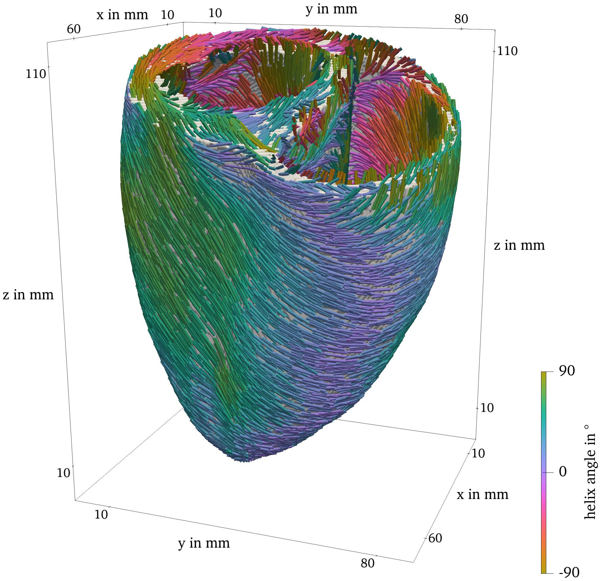
Figure 3: Ventricle geometry with fiber direction, colored by the fiber helix angle.
While the projection matrix ${{\underline{{P}}}}$ is
managed by the Model class, see
section 4.2, the diffusion matrix
${{\bm{{D}}}}$ and the handling of the spatial
derivatives is implemented in the Geometry class. The most important
things the Geometry class takes care of, are:
- Initialization of the computational grid, along with the strides and pointers, which are important for efficient computing;
- Computation of the entries of the diffusion tensor, based on the main directions of diffusion and the respective diffusion values;
- Computation and storage of the weights for the stencils of the numerical spatial derivatives (section 2.3) respecting the Neumann boundary conditions; and
- Handling the upper bound for the time step due to the CFL condition (section 2.2).
The Geometry class is a base class and should not be used directly to
construct a computational domain. Instead, there are several subclasses,
each representing a different type of diffusion or extrinsic shape. An
overview of the Geometry subclasses is given in
Table 2.
| class | description | dim $N$ | points in stencil |
|---|---|---|---|
Geometry_Iso | isotropic diffusion | 1..3 | $2N+1$ |
Geometry_ND | isotropic diffusion in higher dimensions (Cloet et al., 2023) | $N\in\mathbb{N}$ | $2N+1$ |
Geometry_OrtAniso | orthotropic diffusion | 2..3 | $\begin{cases}9 & N=2 \\ 19 & N=3\end{cases}$ |
Surface | 2D domain with extrinsic curvature | 2 | 9 |
QuadricSurface | quadric surface with rotated parallel fibers | 2 | 9 |
Ellipsoid | ellipsoidal surface with rotated parallel fibers | 2 | 9 |
Hyperboloid | hyperboloidal surface with rotated parallel fibers | 2 | 9 |
Paraboloid | paraboloidal surface with rotated parallel fibers (Dierckx et al., 2013) | 2 | 9 |
Table 2: Overview of tissue geometries supported by Ithildin.
The Geometry_ND class is a subclass of Geometry_Iso and the
Ellipsoid, Hyperboloid, and Paraboloid classes are subclasses of
QuadricSurface.
The details on how the extrinsic and intrinsic curvature affect the diffusion tensor and hence the weights for the discretized differential operator, are discussed in the documentation of the code. There, the different ways to initialize the available domain types are given as well.
Note that some additional features are implemented in the Geometry
class, that do not have a direct link with the diffusion term, such as
inhomogeneities (section 4.3) and
filament detection (section 4.7).
Reaction term
The Model class serves as the base class for all cardiac
electrophysiology models in the Ithildin framework. It encapsulates
common functions and variables used across different models. Key
features of the Model class include:
- Implementation of the reaction term ${{\underline{{r}}}}{{\left( {{\underline{{u}}}} \right)}}$ in the reaction-diffusion equation.
- Storage of model-specific metadata such as relevant citations.
- Handling of variable-related information, including their names, indices, and resting values.
- Management of the values of the projection matrix ${{\underline{{P}}}}$.
Derived classes extend the Model class to implement specific cardiac
electrophysiology models in the reactionterm function.
An overview of the cell models that are currently included in the source code of this project is provided in Table 3. More models may be added as additional classes.
| class | description | #vars | references |
|---|---|---|---|
Model_1VarPoly | one-variable polynomial model | 1 | |
Model_AP | Aliev-Panfilov, continuous epsilon | 2 | Aliev & Panfilov (1996) |
Model_AP2 | Aliev-Panfilov, discontinuous epsilon | 2 | Aliev & Panfilov (1996) |
Model_AP3 | Aliev-Panfilov, discontinuous epsilon, simple recovery | 2 | Aliev & Panfilov (1996); Pravdin et al. (2015); Dierckx et al. (2015) |
Model_AP4 | Aliev-Panfilov, smoothened epsilon, simple recovery | 2 | Aliev & Panfilov (1996); Pravdin et al. (2015); Dierckx et al. (2015) |
Model_BO | Bueno-Orovio 2008 4 var | 4 | Bueno-Orovio et al. (2008) |
Model_Ba | Barkley | 2 | Barkley (1991) |
Model_FHNa | FitzHugh-Nagumo (a), 2 var | 2 | FitzHugh (1961); Nagumo et al. (1962) |
Model_FHNb | FitzHugh-Nagumo (b), 2 var | 2 | FitzHugh (1961); Nagumo et al. (1962) |
Model_FHNc | FitzHugh-Nagumo (c), 2 var | 2 | FitzHugh (1961); Nagumo et al. (1962) |
Model_FK | Fenton-Karma 3 var | 3 | Fenton & Karma (1998) |
Model_Kaz | Kazantsev PRE 2003 spiking neuron | 2 | Kazantsev et al. (2003) |
Model_LRI | Luo-Rudy Phase I | 8 | Luo & Rudy (1994) |
Model_MS | Mitchell Schaeffer | 2 | Mitchell (2003) |
Model_SmooKa | Smooth Karma by Marcotte 2017 | 2 | Marcotte & Grigoriev (2017); Byrne et al. (2015); Karma (1993); Karma (1994) |
Model_TP06 | Ten Tusscher & Panfilov 2006 | 19 | ten Tusscher & Panfilov (2006); Niederer et al. (2019) |
Table 3: Overview of cell models included in Ithildin.
The Ithildin framework also introduces several ModelWrapper classes
that provide additional functionality and allow for the combination of
models. These wrappers enable the recording of diffusion terms, reaction
terms, local activation times (LAT), and local deactivation times (LDT)
as additional state variables. This is done by adding code to the
reaction term calculations of the underlying model. The wrappers inherit
from the base ModelWrapper class, which is a wrapper that leaves the
model unchanged. The primary ModelWrapper classes are:
ModelWrapper_RecordDiffusionrecords diffusion terms of selected variables as additional variables.ModelWrapper_RecordReactionrecords reaction terms of selected variables as additional variables.ModelWrapper_RecordActivationTimerecords LAT for selected variables.ModelWrapper_RecordDeactivationTimerecords LDT for selected variables.ModelWrapper_RescaleTimeSpacelinearly rescales the wrapped model in time and space.ModelWrapper_RescaleVarslinearly rescales selected state variables of the wrapped model.
The Model_multi class enables the combination of multiple submodels
into a single model. The behavior of the combined model may vary
depending on the location ${{\bm{{x}}}}$ and is
determined by one of its submodels. Which model is to be used depends on
the integer value of the inhom field, which is used to describe
spatial inhomogeneities, such as obstacles. Inhomogeneities will be
further explained in the following, cf.
section 4.3. This class is particularly
useful for simulating scenarios where different regions of cardiac
tissue exhibit distinct behaviors.
The Ithildin C++ framework provides a structured and modular approach to
modeling cardiac electrophysiology. The Model class serves as the base
for different models, while various ModelWrapper classes and the
Model_multi class offer extended functionalities for recording and
combining different model aspects.
Inhomogeneities
In simulations of cardiac electrophysiology, accurately modeling the spatial properties of the cardiac tissue is essential. Inhomogeneities represent variations in the tissue’s characteristics, such as its electrical conductivity or cellular properties, that influence the propagation of electrical signals.
An inhomogeneity in the Ithildin framework is a distinct region within
the simulation domain with different properties compared to its
surroundings. In the context of cardiac electrophysiology, these
properties could correspond to variations in the electrical
conductivities of cells, cellular properties, or even the absence of
excitable cells altogether. Inhomogeneities are defined by an integer
field called inhom associated with each point in the domain. Grid
points with a non-zero inhom value are considered interior points,
indicating that the reaction-diffusion equation needs to be solved on
these points. If the selected reaction term is a Model_multi (see also
section 4.2), for an inhom value of
$n$, the $n$th submodel will be
used for this point. For example, in Fig. 4,
the inhom field for Sim. 1 is visualized. Two different cell models
are used for the values 1 and 2. The points where inhom has the value
0, are considered exterior points. The set of all interior points is
the physical domain $\Omega$. At the boundary of the
physical domain, Neumann boundary conditions are applied.
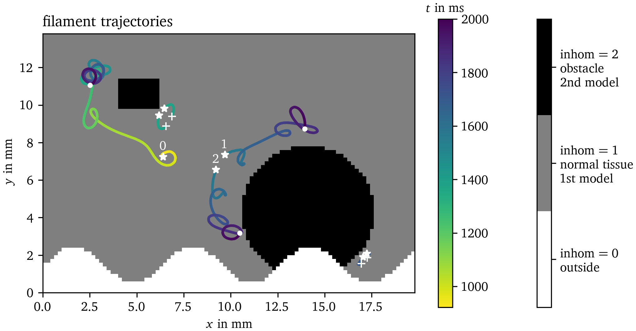
Figure 4: Inhomogeneities in Sim. 1. The field inhom describes
where unexcitable obstacles or exterior points are located with the
value inhom = 0 and which cell model is to be used inside if
inhom > 0. This figure also visualizes the filament trajectories
colored by time, cf. section 4.7. Birth of a
tip is denoted by stars, their deaths by crosses, and tips that are
still around at the end of the simulation by points. The three
trajectories with the longest lifetime are numbered by indices 0 through
2.
To incorporate inhomogeneities into the simulation, the framework provides methods to add them to the domain. These methods allow specifying the shape, location, and properties of each inhomogeneity. For example, a rectangular inhomogeneity could be added by specifying its width, height and location.
Stimulation protocols
Ithildin provides a flexible way to define stimulation protocols using
the Stimulus and Trigger classes, as well as the scheduling
functionality of the Source class.
The Stimulus class enables the specification of temporal and spatial
characteristics of voltage-based or current-based stimuli. It allows
defining which state variables should be affected directly, the
associated values, and whether the stimulus sets the variable directly
or whether it is additive and hence behaving like a current source.
Temporal modulation of stimulus strength is achieved through the
amplitude function, while spatial constraints are managed by the
shape function, an instance of the Shape class.
The Shape class describes a geometric shape via its characteristic
function which can be used to define regions of interest in a simulation
domain. The core principle is that the function evaluates a given
position vector and returns a value: 1 if the position is inside the
defined shape, and 0 if it is outside. However, values in the range
${{\left[ 0,1 \right]}}$ may also be used to create a
smooth transition. A smoothly varying characteristic function may be
useful to create more-realistic stimuli that deposit current in a smooth
profile. This simple yet powerful concept forms the basis for
constructing intricate spatial configurations.
The Shape class provides several pre-defined shape functions, though
additional shapes can easily be added by defining a characteristic
function:
- Ellipsoid: Defined by radii, a center and optionally the Euler angles, this shape represents a general three-dimensional ellipsoid with the specified orientation.
- Sphere: A special case of an ellipsoid where all radii are equal, forming a three-dimensional sphere.
- Ellipse in $xy$-plane: This two-dimensional shape resembles an ellipse lying on the $xy$-plane, defined by radii and a center.
- Cylinder along $z$-axis: Representing a three-dimensional cylinder centered along the $z$-axis, this shape is defined by a radius and a center. In 2D, it defines a disk.
- Rectangular cuboid: Defining a three-dimensional region, this shape is specified by two opposing corner points, creating a cuboid. In 2D, it defines a rectangle.
- Half plane: A plane defined by an origin and an outward normal vector splits the three-dimensional space into a half-space. In 2D, a straight line splits the plane in a similar way.
Characteristic functions can also be loaded from files in the NPY format (Harris et al., 2020). This feature facilitates the incorporation of custom shapes derived from external data sources.
The scheduling functionality via Source::schedule offers the ability
to execute functions at specified points in time during the simulations.
This feature greatly enhances experimental flexibility by allowing the
execution of arbitrary code snippets at chosen moments during
simulations. The scheduler is especially useful for introducing dynamic
changes to the simulation environment, such as modifying stimuli or
conditions mid-simulation.
The Trigger class provides a means to orchestrate actions based on
specific conditions. Triggers encapsulate the decision-making process of
when to execute a particular action, influenced by condition checks and
coordination modes. Different coordination modes allow for the
synchronization of trigger actions across multiple processes,
facilitating complex simulations of activation waves. These modes are to
trigger on each process individually once the condition is met, once the
condition is met in a specific process, once the condition is met in any
process, or once it is true in all processes.
Within the framework of cardiac electrophysiology, triggers are essential for defining stimulation protocols, e.g. for the S1S2 protocol, which is illustrated in Fig. 5: After a first excitation wave passes a sensor position, a second wave is triggered behind a part of the first waveback to stimulate spiral waves.
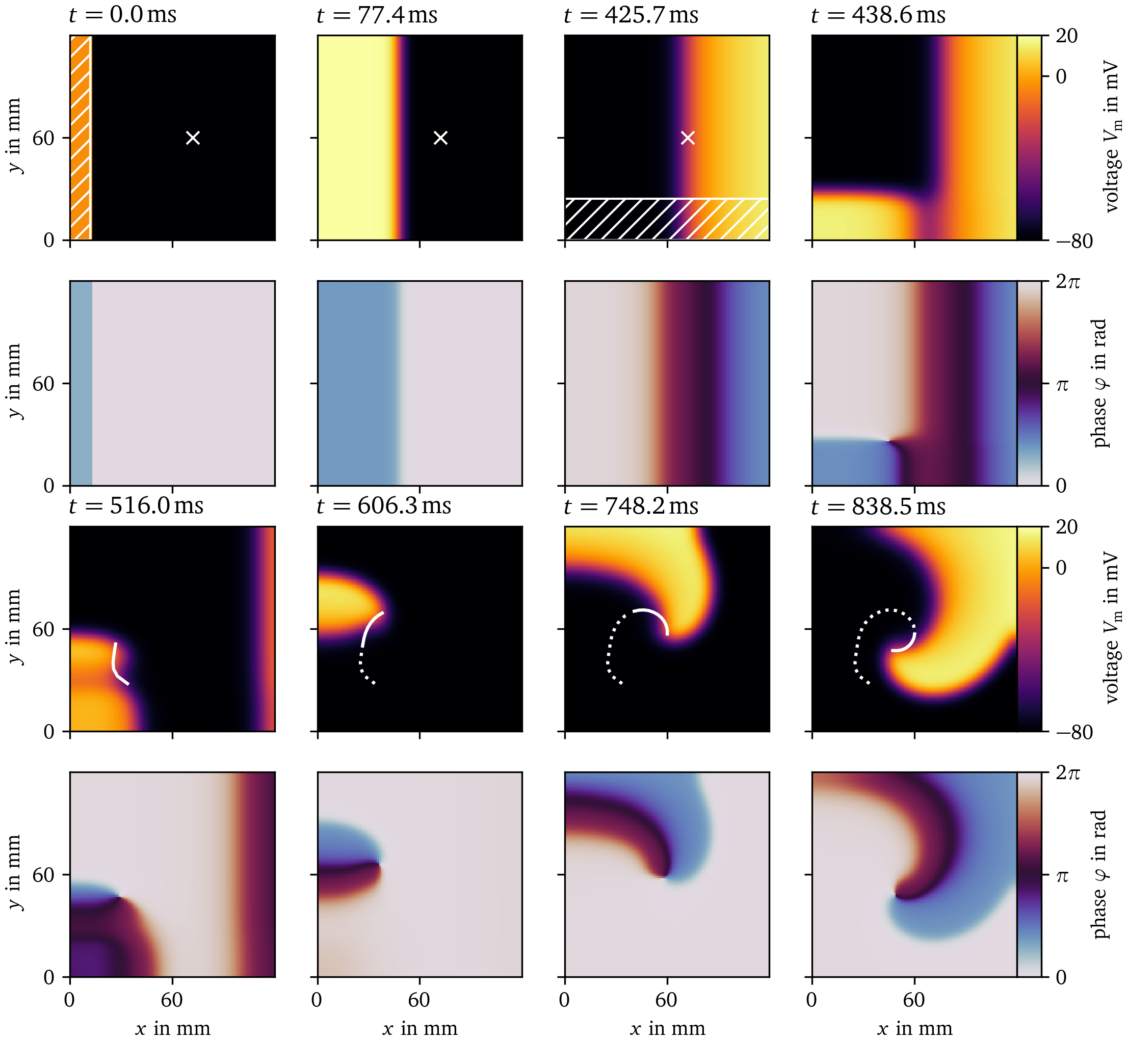
Figure 5: The S1S2 protocol illustrated for Sim. 2. The first and third row display the transmembrane voltage $u$ at selected frames in time, and the second and fourth row the state space phase (Arno et al., 2021; Kabus et al., 2022). The first stimulus is applied in the first frame in the hatched region at the left edge. The sensor location is marked with a cross. Right after the third frame, the sensor triggers the second stimulus in the hatched region at the bottom edge. A spiral wave forms. The phase singularity at the center of the spiral is tracked as the curve, which is dotted for the entire trajectory of the phase singularity, and solid for its trajectory since the previous frame.
Recording temporal evolution of variables at sensor positions
Besides the sensors for triggering stimuli, sensors in the context of this simulation framework are components that monitor and record the state variables of the simulated system at chosen positions during the simulation. We call this the history at a given sensor position.
These sensors are used to gather data about the behavior of the system
at particular time intervals, regulated by the sensorlag parameter.
This parameter controls the frequency at which sensor data is collected,
allowing for flexibility in recording intervals. Notably, the recording
frequency set by sensorlag need not align with the simulation’s time
step or the duration between frames. The data will be recorded at the
first time step after the specified sensorlag duration. This
high-resolution temporal data can be used to study individual points in
the medium in detail.
The recorded data are then written to designated comma separated value (CSV) output files associated with each sensor. These files are used to store the collected data over the course of the simulation.
The first four panels of Fig. 6 contain time traces of the transmembrane voltage $u$, the restitution variable $v$, the recorded value of the diffusion term, and the LAT at a given sensor position for Sim. 1. The times of the three stimuli are indicated by the black vertical lines. The other panels will be explained in the subsequent sections.
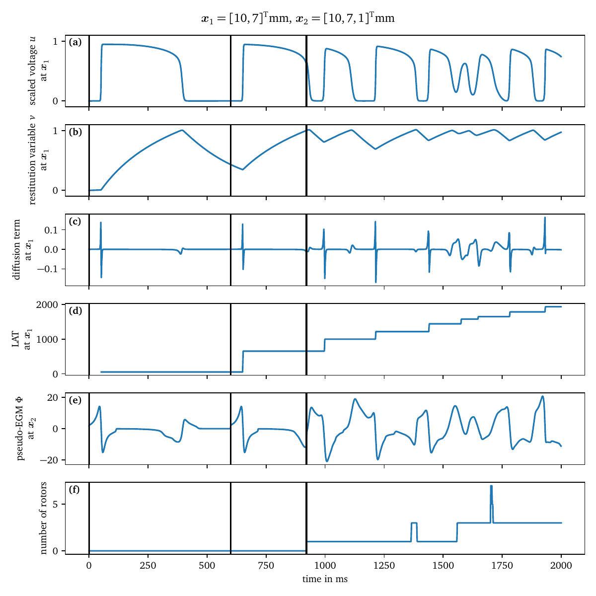
Figure 6: Extracted time traces of Sim. 1. The first two panels (a, b) contain the model variables $u$ and $v$, followed by data computed by model wrappers, namely the diffusion term $\nabla \cdot {{\bm{{D}}}} \nabla u$ (c) and the LAT (d), at an interior point, cf. section 4.5. Panel (e) contains the pseudo-EGM at an exterior point, next to the 2D domain, cf. section 4.6. The last panel (f) contains the number of rotors detected via phase singularities, cf. section 4.7. The black vertical lines indicate times at which a stimulus was applied.
Pseudo-EGMs
The EGM is a measurement of the potential generated by the charge
distribution in cardiac tissue over time at a point in space, outside
the tissue. In theory, this is a measurement of the extracellular
potential ${\Phi_\text{e}}$. However, since Ithildin
is a monodomain solver, the extracellular potential is not part of the
model equations (Clayton et al., 2011). The
code therefore calculates an approximation of the extracellular
potential at points outside the mesh using the Egm class. To obtain
this approximation, the pseudo-bidomain theory is used (Bishop & Plank,
2011). The approximation, referred to as a
pseudo-EGM, uses the simplifications that the intracellular and
extracellular conductivities are proportional, such that there is an
explicit formula to calculate the extracellular potential, and that the
bath conductivity is homogeneous.
The extracellular potential ${\Phi_\text{e}}$ at position ${{\bm{{x}}}}_\text{e}$ over time is then calculated as: $$ {\Phi_\text{e}}{{\left( {{\bm{{x}}}}_\text{e},t \right)}} = \frac{ \tau_\text{e} }{ 4\pi } \int_{\Omega}\mathrm{d}{{\bm{{x}}}}\; \frac{ \nabla \cdot {{\bm{{D}}}} \nabla u({{\bm{{x}}}},t) }{ {{\left\lVert {{\bm{{x}}}}_\text{e} - {{\bm{{x}}}} \right\rVert}} } \qquad{(8)}$$ where $\Omega$ denotes the computational domain, i.e., the simulated heart muscle tissue, $u$ is a state variable of the model representing the transmembrane potential, , which is usually encoded as the first variable in the state vector ${{\underline{{u}}}}$. Furthermore, ${{\bm{{D}}}}$ is the diffusion matrix from the reaction-diffusion equation (Eq. 2), and $\tau_\text{e}$ is a proportionality factor with units ${\mathrm{{m}{s}}}$.
Essentially, the used approximation for the EGM is a convolution of the
diffusion term $\nabla \cdot {{\bm{{D}}}} \nabla u$
for the first variable with a kernel
${{\left\lVert {{\bm{{x}}}}_\text{e} - {{\bm{{x}}}} \right\rVert}}^{-1}$.
Depending on the choice of the diffusion tensor, made by the user in the
Geometry class (section 4.1), a
different prefactor of the integral is required. Hence, the prefactor
$\frac{\tau_\text{e}}{4\pi}$ is user-defined and can
be changed using the function set_prefactor.
The integral in Eq. 8 is discretized and its
calculation is implemented such that the additional amount of storage
and number of calculations is limited as much as possible. For instance,
as the required diffusion term
$\nabla \cdot {{\bm{{D}}}} \nabla V_\text{m}$ is
already computed during the forward stepping of the reaction-diffusion
equation, it can be stored as an additional state variable using a
ModelWrapper_RecordDiffusion and subsequently used in the pseudo-EGM
calculation. This model wrapper is essential for the functioning of the
Egm class and hence is a requirement when setting up a simulation with
pseudo-EGM calculation.
The result is a CSV file with the pseudo-EGM data for each electrode that is defined by the user. The computed pseudo-EGM at a given position for Sim. 1 is displayed in the fifth panel of Fig. 6.
Filaments
Formally, filaments can be understood as a line of wave break, i.e., a line where an activation and recovery surface come together (Clayton et al., 2006; Winfree, 1994). The activation surface can be seen as the wavefront, while the recovery surface can be seen as the waveback. When considering an excitable system in 2D, filaments become tips, being the point of intersection between the activation and recovery curve. Since a point cannot be excited and recovering at the same time, points on a filament are also called phase singularities.
Using this definition of filament points, detection algorithms have been designed. Our code relies on the one described by Fenton & Karma (1998). Additionally, this algorithm has been extended to grids in any dimension, where the generalization of filaments are called superfilaments (Cloet et al., 2023).
The filament point detection algorithm is included in the Geometry
class. Its goal is to compute the points where the wavefront and
waveback meet. While looping over all coordinate planes and grid points,
it is checked whether there is an intersection of isolines in the
adjacent voxel faces of a grid point. The location of the filament point
is then estimated by bi-linear interpolation. An illustrative sketch of
this method is given in Fig. 7.
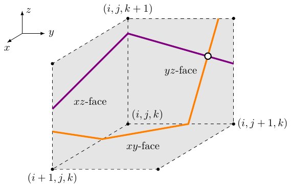
Figure 7: Illustration of the filament point tracking algorithm. Each coordinate plane adjacent to a grid point $(i,j,k)$ is checked for an intersection of two surfaces (purple and orange lines) which are usually isosurfaces of state variables in ${{\underline{{u}}}}$. In this example, a filament point (dot) will be found in the $yz$-face.
The last panel in Fig. 6 displays the number of rotors over time for Sim. 1, which are found via filament detection. It can be seen that at the S2 stimulus, a single rotor is formed, and subsequently pairs of rotors as figure-of-eight spiral pairs.
More details of this process can be seen in Fig. 4 which shows the trajectories of these filaments in Sim. 1 tracked using the Python module for Ithildin. The trajectories are colored by time and the formation of a new tip is denoted by stars and their decay by crosses. Tips that still persist at the final frame of the simulation are indicated by points. The tip trajectory denoted with index 0 is formed by the S1S2 protocol and meanders around the medium. It persists until the end of the simulation. The figure-of-eight spiral wave pair denoted by indices 1 and 2 is formed by a conduction block breaking up. The spiral tip with index 2 runs into the boundary to disintegrate there.
Phase defects
While a phase singularity can be seen as points where all phases meet—in mathematics called a pole, a phase defect is a point at which there is a discrete jump from one phase value to another in an otherwise continuously varying phase. While phase defects are well known in physics, they were only recently identified in excitable media, within linear-core rotors and conduction block regions (Arno et al., 2021; Tomii et al., 2021). Phase defects are lines in 2D and surfaces in 3D.
In Ithildin, the phase defect detection is done with its Python module. For instance, during simulation, Ithildin can record the local activation times (LAT) which can then be used to compute the activation time phase in post-processing (Arno et al., 2021; Kabus et al., 2022). A variety of methods exist to then localize the phase defect (Kabus et al., 2022; Tomii et al., 2021).
Two examples for phase defect detection in Sim. 1 are given in Fig. 8 and Fig. 9. Both display four frames over time of the transmembrane voltage $V_\text{m}$, the activation time phase ${\varphi}$, and the phase defect $\rho$ computed via the cosine method (Kabus et al., 2022; Tomii et al., 2021). In Fig. 8, the phase defect of a single spiral wave is tracked. It can be seen that the phase defect extends due to conduction block such that the spiral wave moves across the domain. In Fig. 9, the break-up of a conduction block line into a figure-of-eight spiral wave pair can be seen. The conduction block line is a phase defect of zero topological charge (Arno et al., 2024a; Goryachev & Kapral, 1996; Mermin, 1979) which, in this case, reaches a critical length breaking apart into two oppositely charged spiral waves with much shorter phase defect lines.
In Fig. 10, we present the final frame of Sim. 4 in ventricular geometry, visualized with ParaView (Ahrens et al., 2005). It is colored by the normalized transmembrane voltage. Both, the classical tip and the phase defect surface are visualized. The spiral waves revolve around the phase defect surfaces.
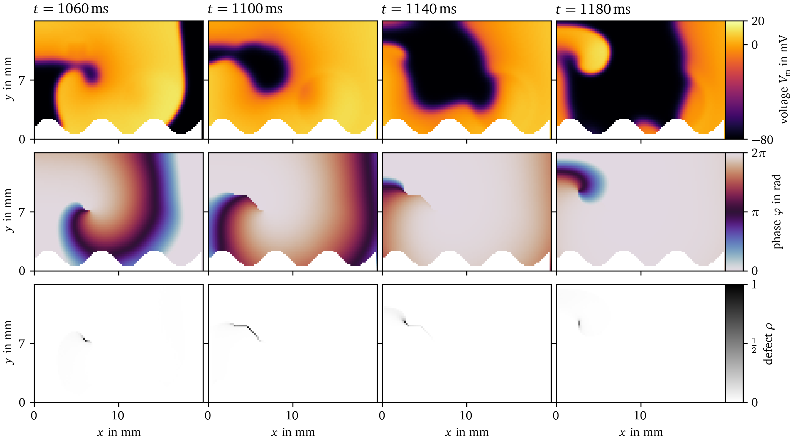
Figure 8: Phase defect detection for a single meandering spiral in Sim. 1. By recording the activation times of the transmembrane voltage $V_\text{m}$ (top row), the activation time phase ${\varphi}$ (Kabus et al., 2022; Tomii et al., 2021) can be computed (middle row). Where this phase is discontinuous, a phase defect is localized. This is visualized as the phase defect density $\rho$ (bottom row). In these four frames, a single rotor is tracked shortly after its formation. Due to conduction block, which can be seen as an extended phase defect line, the spiral moves through the medium. Afterwards, the spiral remains mostly stationary, leading to a shorter phase defect line.
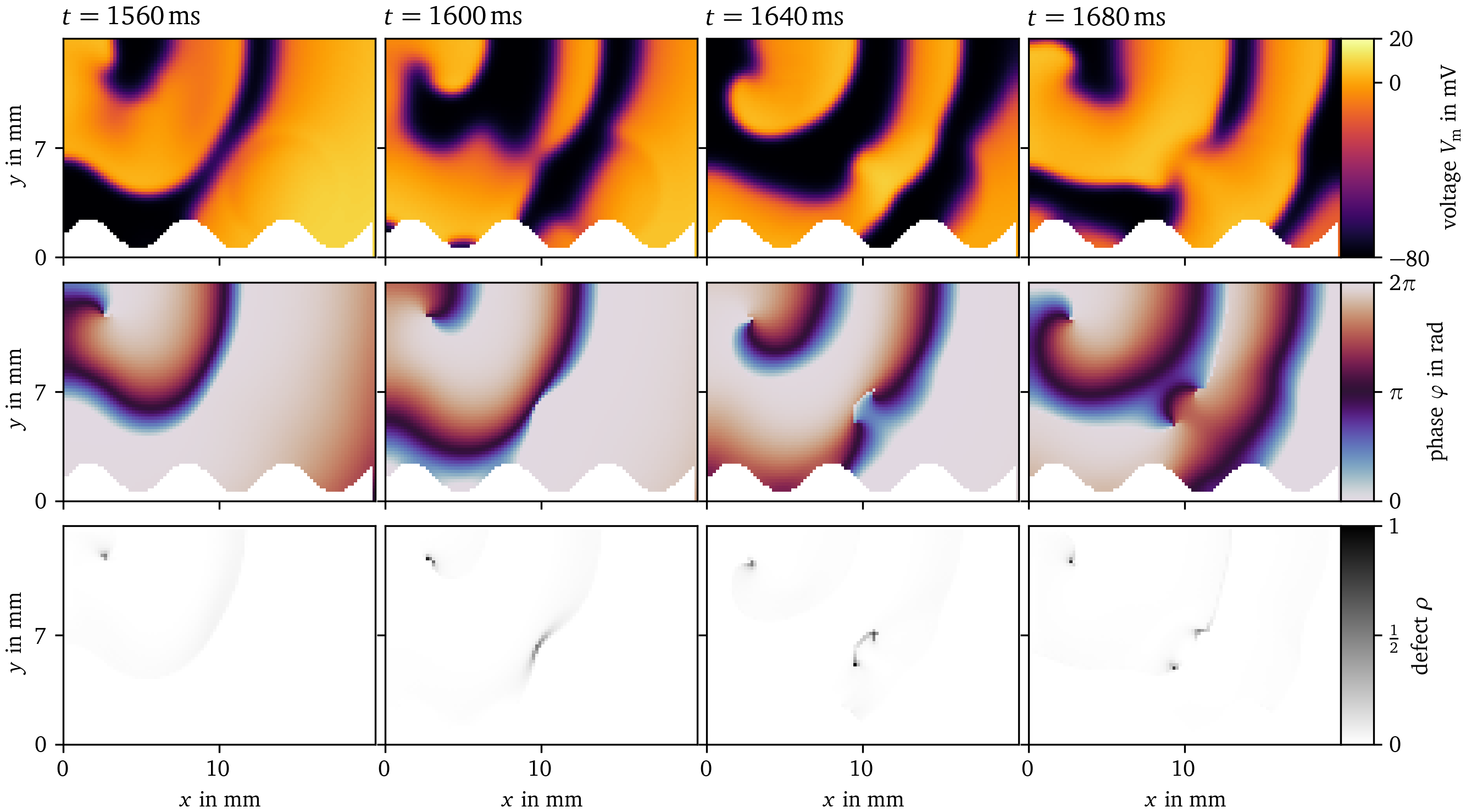
Figure 9: Phase defect detection during figure-of-eight spiral wave pair creation in Sim. 1. Visualization in the same style as Fig. 8. A long conduction block line breaks apart into two rotors.
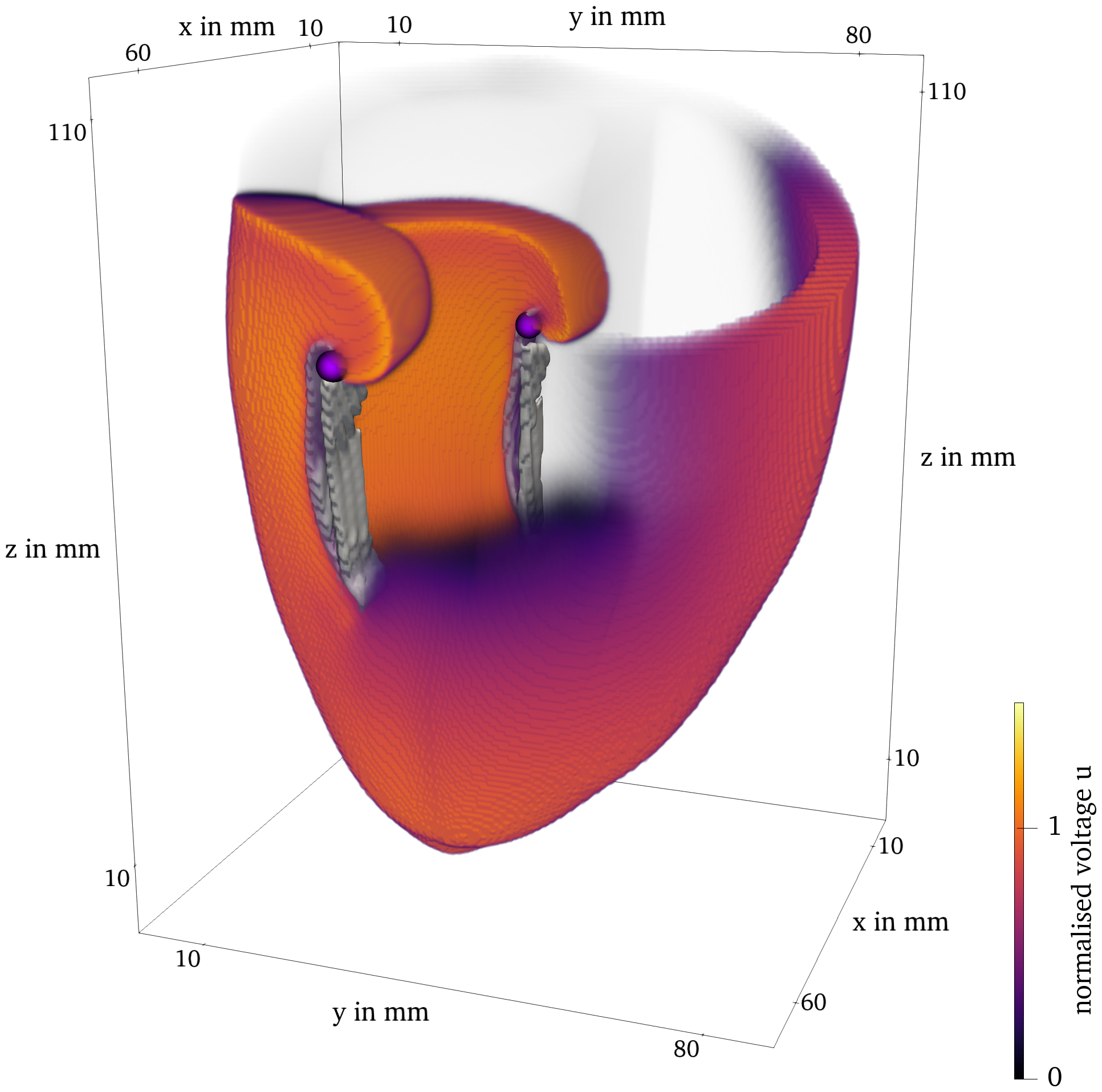
Figure 10: Final frame of Sim. 4 of the BOCF model in ventricle geometry. The classical filament is plotted as the purple lines. The phase defect surface is contained in the gray contour.
Further documentation
More complete documentation of Ithildin can be generated with Doxygen (van Heesch, 2023) and can be also found online, see the data availability statement for details. The documentation contains detailed information on how to get started installing and working with ithildin.
Results
Ithildin is used for numerical experiments in various use cases. For instance, it was used to study the structure of the core of rotors emerging in in-silico cardiac-electrophysiology cell models, leading to the description of phase defect lines (Arno et al., 2021, 2024a, 2024b; Kabus et al., 2022). Also, higher-dimensional rotors waves were simulated and the emerging super-filaments were detected using Ithildin (Cloet et al., 2023). In the creation of novel data-driven cell models using state space expansion, Ithildin was used to generate synthetic training data sets (Kabus, De Coster, et al., 2024).
Five simulations were conducted for this paper to illustrate the features of Ithildin. An overview of the simulations is given in Table 4, along with references to the figures that were generated with these data sets while details on their simulation setup can be found in their C++ code in the appendix.
| simulation | Sim. 1 | Sim. 2 | Sim. 3 | Sim. 4 | Sim. 5 |
|---|---|---|---|---|---|
| cell model | SmooKa | AP | BO | BO | TP06 |
| parameter set | default | default | EPI | EPI | EPI |
| references | 2 | 3 | 4 | 5 | 6 |
| dimensions | 2 | 2 | 2 | 3 | 3 |
| anisotropy type | isotropic | isotropic | isotropic | orthotropic | orthotropic |
| diffusivity $P_{uu}$ | 0.031 | 1.6 | 0.12 | 0.12 | 0.1 |
| ratio $D_\parallel / D_\perp$ | 1.0 | 1.0 | 1.0 | 4.0 | 7.6 |
| inhomogeneities | sphere, rectangle, waves | none | none | biventricular geometry | none |
| grid size | 100×70 | 120×120 | 450×450 | 168×208×231 | various |
| spacing [mm] | $0.2, 0.2$ | $1, 1$ | $0.3, 0.3$ | $0.43, 0.43, 0.5$ | various |
| time step [ms] | 0.1 | 0.1 | 0.1 | 0.1 | various |
| stim. times [ms] | 0, 600, 921 | 0, 426 | 0, 394.1 | 0 | 0 |
| duration [ms] | 2000.1 | 838.6 | 680.1 | 600.1 | 150.0 |
| used in | Figs. 1, 4, 6, 8, 9 | Fig. 5 | Sim. 4 | Figs. 1, 3, 10 | Fig. 11 |
Table 4: Overview of the numerical simulations used in this paper.
Cardiac electrophysiology benchmark
Niederer et al. (2011) proposed a benchmark problem that is now used by the in-silico modelling community to validate and compare cardiac electrophysiology solvers (Campos et al., 2016; Niederer et al., 2011). Ithildin passes the benchmark as implemented in Sim. 5. In the benchmark problem an excitation wave travels through a cuboid-shaped medium following the cell model by ten Tusscher & Panfilov (2006). In Fig. 11, we present the results from the benchmark in a similar way as in the original publication introducing the benchmark (Niederer et al., 2011): Point $P_1={{{{\left[ 0,0,0 \right]}}}^\mathrm{T}}$ is the corner of the cuboid where the stimulus is applied and $P_8={{{{\left[ 20,7,3 \right]}}}^\mathrm{T}}{\mathrm{{m}{m}}}$ the furthest-away opposite corner. Consider the plane going through $P_1$ and $P_8$ as well as $P_{10}={{{{\left[ 0,7,1.5 \right]}}}^\mathrm{T}}{\mathrm{{m}{m}}}$. We call the distance along the long axis of the plane slicing through the cubioid $\xi_1$ and the short axis $\xi_2$. In the panels (a), the LAT on this plane is shown for the benchmark simulation at high and low resolution in space, $\Delta x = {0.1~\mathrm{{m}{m}}}$ and $\Delta x = {0.5~\mathrm{{m}{m}}}$ respectively, at the same temporal resolution $\Delta t = {0.005~\mathrm{{m}{s}}}$. Panel (b) also shows the LAT on the line from $P_1$ to $P_8$ for the different spatial resolutions $\Delta x \in {{\left\{{0.1~\mathrm{{m}{m}}}, {0.2~\mathrm{{m}{m}}}, {0.5~\mathrm{{m}{m}}} \right\}}}$ at the same temporal resolution. In panel (c), the LAT value at $P_8$ is compared across all the combinations of spatial and temporal resolution. Just like for most other solvers which are compared in the benchmark paper, it can be seen that at the coarsest spatial resolution, the excitation wave is slowed down significantly in the transversal direction (Niederer et al., 2011). Similarly to the other finite-difference solvers, the simulation fails at $\Delta t = {0.05~\mathrm{{m}{m}}}$ and $\Delta x = {0.1~\mathrm{{m}{m}}}$ (Niederer et al., 2011), due to numerical instability. When a check of the CFL condition is enabled (Eq. 5), Ithildin suggests to lower $\Delta t$ to given this spatial resolution, leading to a simulation at which no instability is observed.
Panel (d) of Fig. 11 shows the speed-up in computation time from parallelization by comparing the computation time for Sim. 5 at $\Delta x = {0.2~\mathrm{{m}{m}}}$ and $\Delta t = {0.01~\mathrm{{m}{s}}}$ on an 8-core Intel i7-10875H processor using 1, 2, 4, and 8 processes. In the double-logarithmic plot, it can be seen with linear regression that the computational speed increases almost linearly going from one to four processes, $t_\text{sim} \propto N_\text{proc}^{-p}$ with $p \approx 1$. Going to eight processes leads to diminishing returns, resulting in a smaller speed-up in computational time, as the overhead due to the boundary-exchange between processes grows. On this system using eight processes, at $\Delta x = {0.2~\mathrm{{m}{m}}}$ and $\Delta t = {0.01~\mathrm{{m}{s}}}$, solving the benchmark problem takes ${65.733~\mathrm{s}}$ of computation time in Ithildin, while it takes ${611.231~\mathrm{s}}$ in cbcbeat (Rognes et al., 2017). For both codes, we have turned off output to the disk and included the initial setup of the problem, such as compilation and memory allocation.
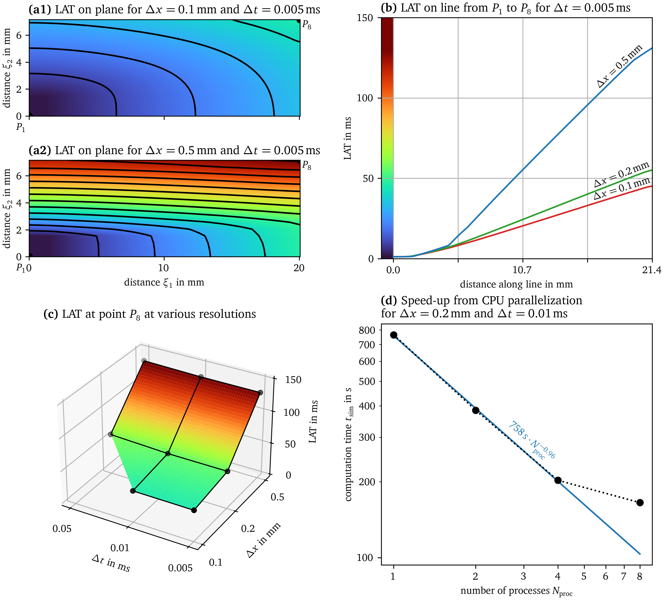
Figure 11: Results of the cardiac electrophysiology benchmark. The benchmark was proposed by Niederer et al. (2011) and is implemented in Sim. 5. To ease comparisons with the paper introducing the benchmark, we present our results in a similar style. In panels (a)-(c), we present the LAT in the medium at different spatial and temporal resolutions. Coloring according to LAT is consistent across these panels. In panel (d), we measure the computational speed of Ithildin at different number of used processes. A linear fit is shown in the double-logarithmic plot which excludes the data point at $N_\text{proc} = 8$.
Discussion
The Ithildin framework is a tool for the simulation of cardiac
electrophysiology. The code offers a number of assets that allow for
simulations targeting a variety of phenomena. For example, there are
many instances available to set the local anisotropy of the myocardium
via the Geometry class. Please refer to the example presented in
section 4.1 for further details. The
Geometry class also allows for the simulation and filament tracking in
a domain with an arbitrary number of spatial dimensions (Arno et al.,
2021, 2024a,
2024b; Cloet et al.,
2023; Kabus et al.,
2022).
These include the ability to define inhomogeneities, which can be used to model domains of any shape and with any kind of obstacles. This is used in Sim. 1 and Sim. 4. Furthermore, the user can define a variety of stimulation protocols, of which some are showcased in the example simulations. We also note the following options: EGM calculation, the possibility of recording the temporal evolution of variables at sensor positions, and the Python module for post-processing and analysis.
It is evident that Ithildin represents but one instance of software designed for the simulation of cardiac electrophysiology. Another finite-differences solver is BeatBox (Antonioletti et al., 2017), which also relies on domain splitting. A non-exhaustive list of examples of established simulation software based on the finite element method (FEM) are Chaste (Cooper et al., 2020), openCARP (Plank et al., 2021), lifex-ep (Africa et al., 2023), cbcbeat (Rognes et al., 2017), GEMS (Arens et al., 2018), CEPS (CARMEN, 2024), and simcardems (Finsberg et al., 2023). Besides the methods of finite differences, elements, and volumes, approaches from computational fluid dynamics such as the lattice Boltzmann method may be used (Campos et al., 2016). Several of these packages have more advanced features than our software. In addition, some have broader applications than cardiac electrophysiology. More software can be found in (Niederer et al., 2011).
Limitations of our software are the fact that, in the context of cardiac electrophysiology, Ithildin only supports the monodomain model as it is a reaction-diffusion problem conforming with Eq. 2, and the fact that the domain decomposition happens solely in one coordinate direction. Further limitations are that Ithildin is fundamentally voxel-based and hence does not support tetrahedral meshes, and that only Neumann boundary conditions are implemented. Additionally, it is only maintained by a small research team. This paper serves to enhance the visibility of the software and to invite fellow cardiac modelers to use and contribute to the project. We believe that the GitLab environment is an effective medium for facilitating interaction between users, identifying issues and suggesting improvements.
Our work with Ithildin has demonstrated its ability to study complex wave patterns in cardiac tissue (Arno et al., 2021, 2024a, 2024b; Cloet et al., 2023; Kabus et al., 2022; Kabus, De Coster, et al., 2024), but it is important to acknowledge the limitations of the fully explicit numerical scheme used: High resolution in time and space may be required for numerical stability. Nevertheless, there are use cases where Ithildin is practical in the context of clinical applications. For example, it can be used to study rotor waves and their implications for cardiac function, which have important implications for diagnosing and treating cardiac diseases. Additionally, Ithildin can be used to develop new models or simulations that are tailored to specific experimental conditions or clinical scenarios.
Conclusion
In this work, we introduced Ithildin, an open-source library that allows for numerical simulation and analysis of rotor waves. We demonstrated the versatility of Ithildin through a series of simulations, including spiral break-up in the Smooth-Karma model, the S1S2 protocol in the AP96 model, and 2D and 3D spiral waves in the BOCF model in ventricular geometry.
Our simulations highlighted several key features of Ithildin, such as the different implemented geometries and reaction terms, inhomogeneities, and stimuli, as well as recording data such as the pseudo-EGM or filament trajectories. These findings contribute to the growing understanding of rotor waves in cardiac electrophysiology and have the potential to inform future experimental and theoretical studies.
Overall, our work demonstrates the power of Ithildin as a tool for studying complex wave patterns in cardiac tissue. We hope that this library will be useful to researchers seeking to better understand the dynamics of rotor waves and their implications for cardiac function.
Data availability
The source code of version 3.5.1 of the Ithildin software implemented for this paper is publicly available at https://gitlab.com/heartkor/ithildin and has been archived on Zenodo (DOI: 10.5281/zenodo.12799245). This archive also contains the data generated by the simulations used throughout this paper. Documentation of the code is publicly available at https://heartkor.gitlab.io/ithildin/.
Appendix
This section contains C++ code to run the four simulations that are used throughout this paper. An overview of their parameters is given in Table 4.
Sim. 1: Spiral break-up in the Smooth-Karma model
This is the source code to the Ithildin simulation used as the main example throughout this paper.
#include "ithildin.h"

int main(int argc, char** argv){
    Mpiclass mpi(argc, argv);

    // define model
    Model_SmooKa model1;

    // define model for obstacles
    Model_SmooKa model2;
    model2.hidden_eps *= 1.5;

    // rescale time and space
    const float scale_time = 2.4; // ms/t.u.
    const float scale_space = 0.273; // mm/s.u.
    ModelWrapper_RescaleTimeSpace model1a{
        &model1, scale_time, scale_space, 2,
    };
    ModelWrapper_RescaleTimeSpace model2a{
        &model2, scale_time, scale_space, 2,
    };

    // rescale u to voltage, such that: u is in range [0, 1]
    const float ucrit = 0.5;
    const float ustim = 0.75;
    ModelWrapper_RescaleVars model1b{&model1a, "u", 0.25, 0.};
    ModelWrapper_RescaleVars model2b{&model2a, "u", 0.25, 0.};

    // record diffusion term for EGMs
    ModelWrapper_RecordDiffusion model1c{&model1b};
    model1c.record("u");
    ModelWrapper_RecordDiffusion model2c{&model2b};
    model2c.record("u");

    // record local activation time
    ModelWrapper_RecordActivationTime model1d{&model1c};
    model1d.record("u", ucrit);
    ModelWrapper_RecordActivationTime model2d{&model2c};
    model2d.record("u", ucrit);

    // combine models
    Model_multi model{{&model1d, &model2d}};

    // geometry parameters
    const size_t Nx = 100;
    const size_t Ny = 70;
    const float dx = 0.2;
    const float dy = dx;
    const float Lx = Nx*dx;
    const float Ly = Ny*dy;

    // set up geometry
    vector<int> size{Nx, Ny, 1};
    vector<float> deltas{dx, dy, 1.};
    Geometry_Iso geom{&mpi, size, deltas, &model};
    geom.add_inhom(
            Shape::Sphere(0.25*Ly, {0.7*Lx, 0.3*Ly}), 2
    );
    geom.add_inhom(
            Shape::Rect({0.2*Lx, 0.7*Ly}, {0.3*Lx, 0.8*Ly}), 2
    );
    geom.add_inhom(Shape([&](vector<float> p) {
        return p[1] < 0.1*Ly*(1. + 0.7*sin(14.*p[0]/Ly));
    }, "waves"), 0);

    // set up simulation and timing
    const int Nframe = 100; // number of frames
    const float framedur = 20.; // time between frames
    const float sampledur = 2.; // sampling time for time traces
    Sim sim{framedur, Nframe, &mpi, &model, &geom, "everything", 0};

    // filament tracking
    model.define_tip("u", ucrit, "v", 0.95);
    sim.enable_filament_recording(0, sampledur);

    // recording temporal data at a specific location
    sim.add_history_point({0.5*Lx, 0.5*Ly});
    sim.sensorlag = sampledur;

    // record EGMs
    sim.add_egm_electrode({0.5*Lx, 0.5*Ly, 1}, sampledur, "diffusu");
    const float lambda = 0.3; // proportionality factor between \
        // intra- and extracellular conduction matrix
    const float beta = 1e5; // 1/m; area-to-volume ratio
    const float capacitance = 1e-2; // F/m²; specific cell \
        // membrane capacitance
    const float conductivity = 0.5; // S/m; lumped conductivity
    for(Egm* egm : sim.egm_collection) {
        egm->construct_kernel(lambda, beta, capacitance, conductivity);
    }

    // set up stimulus protocol
    Source sour(&model, &geom, &mpi, &sim);
    sour.set_val("u", ustim);

    // S0: initial stimulus
    sour.stimulate(Shape::Rect({0, 0}, {0.1*Lx, Ly}));

    // wait until S1S2 protocol starts
    const float timeS1 = 600.; // ms
    sour.schedule.emplace(timeS1, [&]() {
        // S1: first stimulus of S1S2
        sour.stimulate(Shape::Rect({0, 0}, {0.1*Lx, Ly}));

        // S2: second stimulus of S1S2
        sour.setupS2(Point::Phys(&geom, &mpi, 0.5*Lx, 0.9*Ly), 0, ucrit,
            [&]() -> void {
                sour.stimulate(Shape::Rect({0, 0}, {Lx, 0.5*Ly}));
            }
        );
    });

    return sim.run(&sour);
}
Sim. 2: 2D spiral wave in the AP96 model
This example illustrates the S1S2 protocol in an easy-to-interpret setting.
#include "ithildin.h"

int main(int argc, char** argv){
    Mpiclass mpi(argc, argv);

    Model_AP model0(0.15, 0.002, 8, 0.2, 0.3, 20);

    // rescale time and space [@aliev1996simple]
    const float scale_time = 12.9; // ms/t.u.
    const float scale_space = 1.; // mm/s.u.
    ModelWrapper_RescaleTimeSpace model{
        &model0, scale_time, scale_space, 2,
    };

    vector<int> size = {120, 120, 1};
    vector<float> dx = {1.0, 1.0, 1.0};
    float Lx = size[0]*dx[0];
    float Ly = size[1]*dx[1];
    Geometry_Iso geom{&mpi, size, dx, &model};

    float framedur = 1.*scale_time;
    int Nframe = 65;
    Sim sim{framedur, Nframe, &mpi, &model, &geom, "s1s2", 0};
    sim.enable_filament_recording(0, framedur);

    Source sour{&model, &geom, &mpi, &sim};
    sour.set_val("u", 0.75);

    // S1
    sour.stimulate(Shape::Rect({0, 0}, {0.1f*Lx, Ly}));

    // S2
    const Point sensor = Point::Phys(&geom, &mpi, 0.6f*Lx, 0.5f*Ly, 0);
    LOG("sensor", sensor.get_phys());
    sour.setupS2(sensor, 0, 0.5, [&]() -> void {
        sour.stimulate(Shape::Rect({0, 0}, {Lx, 0.2f*Ly}));
    });

    return sim.run(&sour);
}
Sim. 3: 2D spiral wave in the BOCF model
This simulation is used to get an initial state for a 3D simulation in ventricular geometry in the following example.
#include "ithildin.h"

int main(int argc, char** argv){
    Mpiclass mpi(argc, argv);

    // define model
    Model_BO modelbo{1};
    const float ucrit = 0.5;
    const float ustim = 1.0;

    // record local activation time
    ModelWrapper_RecordActivationTime model{&modelbo};
    model.record("u", ucrit);

    // set up geometry
    vector<int> size{450, 450, 1};
    vector<float> dx{0.3, 0.3, 1.};
    const float Lx = size[0]*dx[0];
    const float Ly = size[1]*dx[1];
    Geometry_Iso geom = Geometry_Iso(&mpi, size, dx, &model);

    // set up simulation and timing
    const float framedur = 20.;
    const int Nframe = 34;
    Sim sim{framedur, Nframe, &mpi, &model, &geom, "bocf2d", 0};

    // set up stimulus protocol
    Source sour(&model, &geom, &mpi, &sim);
    sour.set_val("u", ustim);

    // S1: first stimulus of S1S2
    sour.stimulate(Shape::Rect({0, 0}, {0.1*Lx, Ly}));

    // S2: second stimulus of S1S2
    const Point sensor = Point::Phys(&geom, &mpi, 0.75*Lx, 0.5*Ly);
    LOG("sensor", sensor.get_phys());
    sour.setupS2(sensor, 0, ucrit, [&]() -> void {
        sour.stimulate(Shape::Rect({0, 0}, {0.75*Lx, 0.75*Ly}));
    });

    return sim.run(&sour);
}
Sim. 4: 3D spiral wave in the BOCF model
This 3D spiral wave is stimulated by extending a 2D spiral wave and placing it on ventricular geometry.
#include "ithildin.h"

int main(int argc, char** argv){
    Mpiclass mpi(argc, argv);

    // choose model
    Model_BO modelbo{1};
    const float ucrit = 0.5;
    const float ustim = 1.0;

    // record local activation time
    ModelWrapper_RecordActivationTime model{&modelbo};
    model.record("u", ucrit);

    // set up geometry
    vector<float> Ds {1, 0.25, 0.25};
    vector<int> size {168, 208, 231};
    vector<float> deltas {0.43, 0.43, 0.5};
    Geometry_OrtAniso geom{
        size, deltas, "ventricles", &model, Ds, &mpi,
    };

    // set up simulation
    float framedur = 20.;
    int Nframe = 30;
    Sim sim{framedur, Nframe, &mpi, &model, &geom, "bocf3d", 0};

    // filament tracking
    sim.enable_filament_recording(0, framedur);

    // set up stimuli
    Source sour{&model, &geom, &mpi, &sim};

    // transform 2D simulation onto 3D ventricles, PD on RV
    NDArray<float> transform; transform.read("bocf2d3d.transform.npy");
    NDArray<float> vars = sour.read_from_stem("bocf2d_0", 34);
    const vector<size_t> shape{
        vars.get_shape(0), size[0], size[1], size[2],
    };
    vars = vars.interpolate(&mpi, shape,
        [&transform](std::vector<float> x){
            if(x.size() != 4) { ERROR("invalid shape"); }
            std::vector<float> z{1., x[1], x[2], x[3]};
            std::vector<float> y(4, 0);
            for(size_t i=0; i<4; i++) {
                for(size_t j=0; j<4; j++) {
                    y[i] += transform(i,j)*z[j];
                }
            }
            return std::vector<float>{x[0], y[1], y[2], y[3]};
        }
    );
    sour.set_frame(vars);

    return sim.run(&sour);
}
Sim. 5: Cardiac electrophysiology benchmark
This is the benchmark problem as proposed by Niederer et al. (2011) using the cell model by ten Tusscher & Panfilov (2006).
#include "ithildin.h"

int main(int argc, char** argv){
    std::vector<float> arg = strings_to_floats(argc, argv);
    Mpiclass mpi(argc, argv);

    // arg 1: serial number
    const int serialnr = (arg.size() > 1) ? round(arg.at(1)) : 0;
    MASTER_INFO("serialnr", serialnr);

    // arg 2: discretization {0.1, 0.2, 0.5}
    const float dx = (arg.size() > 2) ? arg.at(2) : 0.2; // mm

    // arg 3: PDE time steps {0.005, 0.01, 0.05}
    const float dt = (arg.size() > 3) ? arg.at(3) : 0.05; // ms

    // define model
    Model_TP06 model_tp06;
    ModelWrapper_RecordActivationTime model{&model_tp06};
    model.record("V", 0);

    // constants
    const float C_m = 0.01; // µF/mm² (membrane capacitance)
    const float chi = 140; // 1/mm (surface-to-volume ratio)

    // diffusivities intra/extra longitudinal/transversal
    const float scale = 1 / (chi * C_m); // mm³/µF
    const float Dil = scale*0.17; // mm²/ms
    const float Dit = scale*0.019; // mm²/ms
    const float Del = scale*0.62; // mm²/ms
    const float Det = scale*0.24; // mm²/ms

    // diffusivities longitudinal/transversal
    const float Dl = Dil*Del / (Dil+Del); // mm²/ms
    const float Dt = Dit*Det / (Dit+Det); // mm²/ms

    // diffusivity tensor only scales, Pmat stores magnitude
    vector<float> D{1., Dt/Dl, Dt/Dl}; // 1
    model.set_Pmat(Dl); // mm²/ms

    // domain size
    const float Lx = 20; // mm
    const float Ly = 7; // mm
    const float Lz = 3; // mm

    // set up geometry
    vector<float> deltas{dx, dx, dx};
    vector<int> size{
        int(Lx/deltas[0])+1, int(Ly/deltas[1])+1, int(Lz/deltas[2])+1,
    };
    vector<float> tissue_angles{0., 0.};
    vector<float> diffpars{1, 1, 0};
    Geometry_OrtAniso geom{
        size, deltas, &model, tissue_angles, diffpars, D, &mpi,
    };

    // limit output
    for(size_t ivar=0; ivar<model.get_Nvar(); ivar++)
    { geom.set_bwritevar(ivar, 0); }
    geom.set_bwritevar(model.get_ivar("V"), 1);
    geom.set_bwritevar(model.get_ivar("latV"), 1);

    // set up simulation and timing
    const int Nframe = 15; // number of frames
    const float framedur = 10.; // time between frames in ms
    Sim sim{
        dt, framedur, Nframe, 0, &mpi, &model, &geom,
        "niederer2011benchmark", serialnr, false,
    };

    // set up stimulus
    Source sour(&model, &geom, &mpi, &sim);
    const float I_stim = 50; // mA/cm³ (stimulus current)
    const float i_stim = I_stim * scale; // A/F = V/s = mV/ms
    sour.set_val("V", i_stim); // mV/ms
    sour.stimulate({
            Shape::Rect({0, 0, 0}, {1.5, 1.5, 1.5}),
            1.0, // amplitude factor
            2.0, // ms; duration
            true, // flag: additive stimulus
    });

    return sim.run(&sour);
}
Addenda
Acknowledgments:
We are grateful to Daniël A. Pijnappels, Antoine A.F. de Vries and our other collaborators at the LUMC, as well as Louise Arno, Lore Leenknegt, and Nathan Dermul at KU Leuven in Kortrijk for useful feedback and discussions.
While no generative AI has been used to write the Ithildin source code, generative AI has been used by the authors to aid in the writing of the text, specifically the Large Language Model (LLM) implementations GitHub Copilot, ChatGPT using GPT-3.5 and GPT-4o, as well as Mistral 0.2 via the Ollama software. The authors confirm that they have followed the current ethical publishing practices of PLOS One.
Funding:
DK is supported by KU Leuven grant GPUL/20/012. MC is supported by KU Leuven grant STG/19/007 and FWO-Flanders fellowship, grant 11PMS24N. HD is supported by KU Leuven grant STG/19/007. OB is supported by Agence Nationale de la Recherche grant ANR-IHUA-04. The funders had no role in study design, data collection and analysis, decision to publish, or preparation of the manuscript.
Competing interests:
The authors have declared that no competing interests exist.
Copyright:
© 2024 Kabus et al. This is an open access article distributed under the terms of the Creative Commons Attribution License, which permits unrestricted use, distribution, and reproduction in any medium, provided the original author and source are credited.
Author contributions:
DK: Conceptualization, Methodology, Software, Validation, Formal analysis, Investigation, Data Curation, Writing – original draft, Writing – review & editing, Visualization, Project administration. MC: Methodology, Software, Validation, Formal analysis, Investigation, Data Curation, Writing – original draft, Writing – review & editing, Visualization. CZ: Software. OB: Software. HD: Conceptualization, Software, Resources, Writing – review & editing, Supervision, Project administration, Funding acquisition.
References
Africa, P. C., Piersanti, R., Regazzoni, F., Bucelli, M., Salvador, M., Fedele, M., Pagani, S., Dede’, L., & Quarteroni, A. (2023). Lifex-Ep: A robust and efficient software for cardiac electrophysiology simulations. BMC Bioinformatics, 24(1), 389. https://doi.org/10.1186/s12859-023-05513-8
Ahrens, J., Geveci, B., Law, C., Hansen, C., & Johnson, C. (2005). ParaView: An end-user tool for large-data visualization. The Visualization Handbook, 717, 50038–50031. https://doi.org/10.1016/b978-012387582-2/50038-1
Aliev, R. R., & Panfilov, A. V. (1996). A simple two-variable model of cardiac excitation. Chaos, Solitons & Fractals, 7(3), 293–301. https://doi.org/10.1016/0960-0779(95)00089-5
Antonioletti, M., Biktashev, V. N., Jackson, A., Kharche, S. R., Stary, T., & Biktasheva, I. V. (2017). BeatBox—HPC simulation environment for biophysically and anatomically realistic cardiac electrophysiology. PLOS ONE, 12(5), e0172292. https://doi.org/10.1371/journal.pone.0172292
Arens, S., Dierckx, H., & Panfilov, A. V. (2018). GEMS: A fully integrated PETSc-based solver for coupled cardiac electromechanics and bidomain simulations. Frontiers in Physiology, 9, 1431. https://doi.org/10.3389/fphys.2018.01431
Arno, L., Kabus, D., & Dierckx, H. (2024a). Analysis of complex excitation patterns using Feynman-like diagrams. Scientific Reports, 14(1), 28962. https://doi.org/10.1038/s41598-024-73544-z
Arno, L., Kabus, D., & Dierckx, H. (2024b). Strings, branes and twistons: Topological analysis of phase defects in excitable media such as the heart. In arXiv preprint arXiv:2401.02571. https://doi.org/10.48550/arXiv.2401.02571
Arno, L., Quan, J., Nguyen, N. T., Vanmarcke, M., Tolkacheva, E. G., & Dierckx, H. (2021). A phase defect framework for the analysis of cardiac arrhythmia patterns. Frontiers in Physiology, 12. https://doi.org/10.3389/fphys.2021.690453
Barkley, D. (1991). A model for fast computer simulation of waves in excitable media. Physica D: Nonlinear Phenomena, 49(1-2), 61–70. https://doi.org/10.1016/0167-2789(91)90194-e
Bishop, M. J., & Plank, G. (2011). Bidomain ECG simulations using an augmented monodomain model for the cardiac source. IEEE Transactions on Bio-Medical Engineering, 58(8). https://doi.org/10.1109/TBME.2011.2148718
Bueno-Orovio, A., Cherry, E. M., & Fenton, F. H. (2008). Minimal model for human ventricular action potentials in tissue. Journal of Theoretical Biology, 253(3), 544–560. https://doi.org/10.1016/j.jtbi.2008.03.029
Byrne, G., Marcotte, C. D., & Grigoriev, R. O. (2015). Exact coherent structures and chaotic dynamics in a model of cardiac tissue. Chaos: An Interdisciplinary Journal of Nonlinear Science, 25(3), 033108. https://doi.org/10.1063/1.4915143
Campos, J. O., Oliveira, R. S., dos Santos, R. W., & Rocha, B. M. (2016). Lattice boltzmann method for parallel simulations of cardiac electrophysiology using GPUs. Journal of Computational and Applied Mathematics, 295, 70–82. https://doi.org/10.1016/j.cam.2015.02.008
CARMEN. (2024). Cardiac ElectroPhysiology Simulator (CEPS). IHU Liryc, Inria. https://carmen.gitlabpages.inria.fr/ceps/
Clayton, R., Bernus, O., Cherry, E. M., Dierckx, H., Fenton, F. H., Mirabella, L., Panfilov, A. V., Sachse, F. B., Seemann, G., & Zhang, H. (2011). Models of cardiac tissue electrophysiology: Progress, challenges and open questions. Progress in Biophysics and Molecular Biology, 104(1-3), 22–48. https://doi.org/10.1016/j.pbiomolbio.2010.05.008
Clayton, R., Zhuchkova, E., & Panfilov, A. (2006). Phase singularities and filaments: Simplifying complexity in computational models of ventricular fibrillation. Progress in Biophysics and Molecular Biology, 90(1-3), 378–398. https://doi.org/10.1016/j.pbiomolbio.2005.06.011
Cloet, M., Arno, L., Kabus, D., Van der Veken, J., Panfilov, A. V., & Dierckx, H. (2023). Scroll waves and filaments in excitable media of higher spatial dimension. Physical Review Letters, 131(20), 208401. https://doi.org/10.1103/PhysRevLett.131.208401
Cooper, F. R., Baker, R. E., Bernabeu, M. O., Bordas, R., Bowler, L., Bueno-Orovio, A., Byrne, H. M., Carapella, V., Cardone-Noott, L., Cooper, J., Dutta, S., Evans, B. D., Fletcher, A. G., Grogan, J. A., Guo, W., Harvey, D. G., Hendrix, M., Kay, D., Kursawe, J., Maini, P. K., McMillan, B., Mirams, G. R., Osborne, J. M., Pathmanathan, P., Pitt-Francis, J. M., Robinson, M., Rodriguez, B., Spiteri, R. J., & Gavaghan, D. J. (2020). Chaste: Cancer, Heart and Soft Tissue Environment. Journal of Open Source Software, 5(47), 1848. https://doi.org/10.21105/joss.01848
Courant, R., Friedrichs, K., & Lewy, H. (1928). Über die partiellen Differenzengleichungen der mathematischen Physik. Mathematische Annalen, 100(1), 32–74. https://doi.org/10.1007/BF01448839
Dierckx, H., Arens, S., Li, B.-W., Weise, L. D., & Panfilov, A. V. (2015). A theory for spiral wave drift in reaction-diffusion-mechanics systems. New Journal of Physics, 17(4), 043055. https://doi.org/10.1088/1367-2630/17/4/043055
Dierckx, H., Brisard, E., Verschelde, H., & Panfilov, A. V. (2013). Drift laws for spiral waves on curved anisotropic surfaces. Physical Review E, 88(1), 012908. https://doi.org/10.1103/PhysRevE.88.012908
döt Net, I., Müller, T., Antoniou, P., Aro, E., Smith, T., Evans, C. C., & Ben-Kiki, O. (2023). YAML ain’t markup language, revision 1.2.2. YAML Language Development Team. https://yaml.org/spec/1.2.2/
Euler, L. (1794). Institutiones calculi integralis (Vol. 4). Academia Imperialis Scientiarum.
Fenton, F. H., & Karma, A. (1998). Vortex dynamics in three-dimensional continuous myocardium with fiber rotation: Filament instability and fibrillation. Chaos: An Interdisciplinary Journal of Nonlinear Science, 8(1), 20–47. https://doi.org/10.1063/1.166311
Finsberg, H. N. T., van Herck, I. G. M., Daversin-Catty, C., Arevalo, H., & Wall, S. (2023). simcardems: A FEniCS-based cardiac electro-mechanics solver. Journal of Open Source Software, 8(81), 4753. https://doi.org/10.21105/joss.04753
FitzHugh, R. (1961). Impulses and physiological states in theoretical models of nerve membrane. Biophysical Journal, 1(6), 445–466. https://doi.org/10.1016/s0006-3495(61)86902-6
Gillette, K., Gsell, M. A. F., Prassl, A. J., Karabelas, E., Reiter, U., Reiter, G., Grandits, T., Payer, C., Štern, D., Urschler, M., Bayer, J. D., Augustin, C. M., Neic, A., Pock, T., Vigmond, E. J., & Plank, G. (2021). A framework for the generation of digital twins of cardiac electrophysiology from clinical 12-leads ECGs. Medical Image Analysis, 71, 102080. https://doi.org/10.1016/j.media.2021.102080
Goryachev, A., & Kapral, R. (1996). Spiral waves in chaotic systems. Physical Review Letters, 76(10), 1619–1622. https://doi.org/10.1103/PhysRevLett.76.1619
Graham, R. L., Shipman, G. M., Barrett, B. W., Castain, R. H., Bosilca, G., & Lumsdaine, A. (2006). Open MPI: A high-performance, heterogeneous MPI. 2006 IEEE Int. Conf. On Cluster Computing, 1–9. https://doi.org/10.1109/CLUSTR.2006.311904
Harris, C. R., Millman, K. J., Walt, S. J. van der, Gommers, R., Virtanen, P., Cournapeau, D., Wieser, E., Taylor, J., Berg, S., Smith, N. J., Kern, R., Picus, M., Hoyer, S., Kerkwijk, M. H. van, Brett, M., Haldane, A., Río, J. F. del, Wiebe, M., Peterson, P., Gérard-Marchant, P., Sheppard, K., Reddy, T., Weckesser, W., Abbasi, H., Gohlke, C., & Oliphant, T. E. (2020). Array programming with NumPy. Nature, 585(7825), 357–362. https://doi.org/10.1038/s41586-020-2649-2
Hren, R. (1996). A realistic model of the human ventricular myocardium: Application to the study of ectopic activation [PhD thesis, Dalhousie University]. https://dalspace.library.dal.ca/handle/10222/55139
Hunter, J. D. (2007). Matplotlib: A 2D graphics environment. Computing in Science & Engineering, 9(3), 90–95. https://doi.org/10.1109/MCSE.2007.55
ISO. (2011). ISO/IEC 14882:2011: Information technology — programming languages — C++ (Third, p. 1338). International Organization for Standardization.
ISO. (2014). ISO/IEC 14882:2014: Information technology — programming languages — C++ (Fourth, p. 1358). International Organization for Standardization.
ISO. (2017). ISO/IEC 14882:2017: Programming languages — C++ (Fifth, p. 1605). International Organization for Standardization.
ISO. (2020). ISO/IEC 14882:2020: Programming languages — C++ (Sixth, p. 1853). International Organization for Standardization.
ISO. (2023). ISO/IEC 14882:2023: Programming languages — C++ (Seventh, p. 2101). International Organization for Standardization.
Kabus, D., Arno, L., Leenknegt, L., Panfilov, A. V., & Dierckx, H. (2022). Numerical methods for the detection of phase defect structures in excitable media. PLOS ONE, 17(7), 1–31. https://doi.org/10.1371/journal.pone.0271351
Kabus, D., Cloet, M., Zemlin, C., Bernus, O., & Dierckx, H. (2024). The Ithildin library for efficient numerical solution of anisotropic reaction-diffusion problems in excitable media. PLOS ONE, 19(9), 1–26. https://doi.org/10.1371/journal.pone.0303674
Kabus, D., De Coster, T., de Vries, A. A. F., Pijnappels, D. A., & Dierckx, H. (2024). Fast creation of data-driven low-order predictive cardiac tissue excitation models from recorded activation patterns. Computers in Biology and Medicine, 169, 107949. https://doi.org/10.1016/j.compbiomed.2024.107949
Karma, A. (1993). Spiral breakup in model equations of action potential propagation in cardiac tissue. Physical Review Letters, 71(7), 1103. https://doi.org/10.1103/PhysRevLett.71.1103
Karma, A. (1994). Electrical alternans and spiral wave breakup in cardiac tissue. Chaos: An Interdisciplinary Journal of Nonlinear Science, 4(3), 461–472. https://doi.org/10.1063/1.166024
Kazantsev, V. B., Nekorkin, V. I., Binczak, S., & Bilbault, J. M. (2003). Spiking patterns emerging from wave instabilities in a one-dimensional neural lattice. Physical Review E, 68(1), 017201. https://doi.org/10.1103/PhysRevE.68.017201
Koopsen, T., Gerrits, W., van Osta, N., van Loon, T., Wouters, P., Prinzen, F. W., Vernooy, K., Delhaas, T., Teske, A. J., Meine, M., Cramer, M. J., & Lumens, J. (2024). Virtual pacing of a patient’s digital twin to predict left ventricular reverse remodelling after cardiac resynchronization therapy. Europace, 26(1), euae009. https://doi.org/10.1093/europace/euae009
Li, N., Steiner, J., & Tang, S. (1994). Convergence and stability analysis of an explicit finite difference method for 2-dimensional reaction-diffusion equations. The Journal of the Australian Mathematical Society. Series B. Applied Mathematics, 36(2), 234–241. https://doi.org/10.1017/S0334270000010377
Luo, C., & Rudy, Y. (1994). A dynamic model of the cardiac ventricular action potential. I. Simulations of ionic currents and concentration changes. Circulation Research, 74(6), 1071–1096. https://doi.org/10.1161/01.RES.74.6.1071
Marcotte, C. D., & Grigoriev, R. O. (2017). Dynamical mechanism of atrial fibrillation: A topological approach. Chaos: An Interdisciplinary Journal of Nonlinear Science, 27(9). https://doi.org/10.1063/1.5003259
Mark, E. et al. (2007). Enhancements to the extensible data model and format (XDMF). 2007 DoD High Performance Computing Modernization Program Users Group Conference, 322–327. https://doi.org/10.1109/HPCMP-UGC.2007.30
Mermin, N. D. (1979). The topological theory of defects in ordered media. Reviews of Modern Physics, 51(3), 591–648. https://doi.org/10.1103/RevModPhys.51.591
Mitchell, C. (2003). A two-current model for the dynamics of cardiac membrane. Bulletin of Mathematical Biology, 65(5), 767–793. https://doi.org/10.1016/S0092-8240(03)00041-7
Nagumo, J., Arimoto, S., & Yoshizawa, S. (1962). An active pulse transmission line simulating nerve axon. Proceedings of the IRE, 50(10), 2061–2070. https://doi.org/10.1109/jrproc.1962.288235
Niederer, S. A., Kerfoot, E., Benson, A. P., Bernabeu, M. O., Bernus, O., Bradley, C., Cherry, E. M., Clayton, R., Fenton, F. H., Garny, A., Heidenreich, E., Land, S., Maleckar, M., Pathmanathan, P., Plank, G., Rodríguez, J. F., Roy, I., Sachse, F. B., Seemann, G., Skavhaug, O., & Smith, N. P. (2011). Verification of cardiac tissue electrophysiology simulators using an N-version benchmark. Philosophical Transactions of the Royal Society A: Mathematical, Physical and Engineering Sciences, 369(1954), 4331–4351. https://doi.org/10.1098/rsta.2011.0139
Niederer, S. A., Lumens, J., & Trayanova, N. A. (2019). Computational models in cardiology. Nature Reviews Cardiology, 16(2), 100–111. https://doi.org/10.1038/s41569-018-0104-y
Plank, G., Loewe, A., Neic, A., Augustin, C., Huang, Y.-L., Gsell, M. A. F., Karabelas, E., Nothstein, M., Prassl, A. J., Sánchez, J., Seemann, G., & Vigmond, E. J. (2021). The openCARP simulation environment for cardiac electrophysiology. Computer Methods and Programs in Biomedicine, 208, 106223. https://doi.org/10.1016/j.cmpb.2021.106223
Pravdin, S., Dierckx, H., Markhasin, V. S., & Panfilov, A. V. (2015). Drift of scroll wave filaments in an anisotropic model of the left ventricle of the human heart. BioMed Research International, 2015. https://doi.org/10.1155/2015/389830
Press, W. H. (2007). Numerical recipes 3rd edition: The art of scientific computing. Cambridge university press.
Rognes, M. E., Farrell, P. E., Funke, S. W., Hake, J. E., & Maleckar, M. M. C. (2017). Cbcbeat: An adjoint-enabled framework for computational cardiac electrophysiology. The Journal of Open Source Software, 2(13), 224. https://doi.org/10.21105/joss.00224
Streeter, D. D., Spotnitz, H. M., Patel, D. P., Ross, J., & Sonnenblick, E. H. (1969). Fiber orientation in the canine left ventricle during diastole and systole. Circulation Research, 24(3), 339–347. https://doi.org/10.1161/01.RES.24.3.339
ten Tusscher, K. H. W. J., Hren, R., & Panfilov, A. V. (2007). Organization of ventricular fibrillation in the human heart. Circulation Research, 100(12). https://doi.org/10.1161/CIRCRESAHA.107.150730
ten Tusscher, K. H. W. J., & Panfilov, A. V. (2006). Alternans and spiral breakup in a human ventricular tissue model. American Journal of Physiology-Heart and Circulatory Physiology, 291(3), H1088–H1100. https://doi.org/10.1152/ajpheart.00109.2006
Tolkien, J. R. R. (1954). The Lord of the Rings: The Fellowship of the Ring. Allen & Unwin.
Tomii, N., Yamazaki, M., Ashihara, T., Nakazawa, K., Shibata, N., Honjo, H., & Sakuma, I. (2021). Spatial phase discontinuity at the center of moving cardiac spiral waves. Computers in Biology and Medicine, 130, 104217. https://doi.org/10.1016/j.compbiomed.2021.104217
Trayanova, N. A., Doshi, A. N., & Prakosa, A. (2020). How personalized heart modeling can help treatment of lethal arrhythmias: A focus on ventricular tachycardia ablation strategies in post‐infarction patients. WIREs Systems Biology and Medicine, 12(3). https://doi.org/10.1002/wsbm.1477
van Heesch, D. (2023). Doxygen 1.9.7. Doxygen. https://www.doxygen.nl
Virtanen, P., Gommers, R., Oliphant, T. E., Haberland, M., Reddy, T., Cournapeau, D., Burovski, E., Peterson, P., Weckesser, W., Bright, J., van der Walt, S. J., Brett, M., Wilson, J., Millman, K. J., Mayorov, N., Nelson, A. R. J., Jones, E., Kern, R., Larson, E., Carey, C. J., Polat, İlhan, Feng, Y., Moore, E. W., VanderPlas, J., Laxalde, D., Perktold, J., Cimrman, R., Henriksen, I., Quintero, E. A., Harris, C. R., Archibald, A. M., Ribeiro, A. H., Pedregosa, F., van Mulbregt, P., & SciPy 1.0 Contributors. (2020). SciPy 1.0: Fundamental Algorithms for Scientific Computing in Python. Nature Methods, 17, 261–272. https://doi.org/10.1038/s41592-019-0686-2
Winfree, A. T. (1994). Electrical turbulence in three-dimensional heart muscle. Science, 266, 1003–1006. https://doi.org/10.1126/science.7973648