
This article was previously published in Computers in Biology and Medicine 169 (2024) 107949 (Kabus, De Coster, et al., 2024) and is a chapter of my dissertation.
Authors:
Desmond Kabus1,2 (ORCID: 0000-0002-6965-5211)
Tim De Coster2 (ORCID: 0000-0002-4942-9866)
Antoine A.F. de Vries2 (ORCID: 0000-0002-4787-7155)
Daniël A. Pijnappels2 (ORCID: 0000-0001-6731-4125)
Hans Dierckx1 (ORCID: 0000-0003-0899-8082)
Institutions:
Department of Mathematics, KU Leuven Campus Kortrijk (KULAK), Etienne Sabbelaan 53, 8500 Kortrijk, Belgium
Laboratory of Experimental Cardiology, Leiden University Medical Center (LUMC), Albinusdreef 2, 2333 ZA Leiden, the Netherlands
Correspondence: [email protected]
DOI: 10.1016/j.compbiomed.2024.107949
Keywords:
- data-driven modelling
- surrogate modelling
- machine learning
- digital twin
- excitable media
- cardiac electrophysiology
- optical voltage mapping
Highlights:
- Models of excitation waves can be created in minutes from experiment to fitting.
- One variable in space and time is sufficient to create a working excitation model.
- A polynomial can predict excitation waves based on useful extracted features.
- Spiral waves in heart muscle tissue can be predicted from focal wave data.
Abstract:
Excitable systems give rise to important phenomena such as heat waves, epidemics and cardiac arrhythmias. Understanding, forecasting and controlling such systems requires reliable mathematical representations. For cardiac tissue, computational models are commonly generated in a reaction-diffusion framework based on detailed measurements of ionic currents in dedicated single-cell experiments.
Here, we show that recorded movies at the tissue-level of stochastic pacing in a single variable are sufficient to generate a mathematical model. Via exponentially weighed moving averages, we create additional state variables, and use simple polynomial regression in the augmented state space to quantify excitation wave dynamics. A spatial gradient-sensing term replaces the classical diffusion as it is more robust to noise. Our pipeline for model creation is demonstrated for an in-silico model and optical voltage mapping recordings of cultured human atrial myocytes and only takes a few minutes.
Our findings have the potential for widespread generation, use and on-the-fly refinement of personalised computer models for non-linear phenomena in biology and medicine, such as predictive cardiac digital twins.
Introduction
A wide variety of phenomena qualify as excitable systems, such as epidemics (Noble, 1974) or electrical excitation in the brain (Bressloff, 2014) or heart (Clayton et al., 2011). Reliable and accurate mathematical modelling of these systems is necessary to forecast their evolution in time. These predictions are useful for decision making to steer these systems to a desired state.
To diagnose and treat heart rhythm disorders, a common health burden, the scientific community is creating sophisticated models for different processes in the heart with the goal of building a digital twin of each patient’s heart, i.e., a full recreation of their heart in the computer (Niederer et al., 2019; Trayanova et al., 2020). One of them is the contraction of the heart, which is controlled by excitation waves travelling through the myocardium (Clayton et al., 2011). An in-silico model of cardiac tissue electrophysiology is a mathematical model that is able to describe the dynamics of the excitation patterns (Clayton et al., 2011). Typically, in-silico models for cardiac electrophysiology fall into one of two categories. On the one hand, there are the mathematical models that focus mostly on the overall dynamics in the tissue (Aliev & Panfilov, 1996; Barkley, 1991; Bueno-Orovio et al., 2008; Fenton & Karma, 1998; FitzHugh, 1961; Marcotte & Grigoriev, 2017; Nagumo et al., 1962). While most of these models have continuous state variables, there are also cellular automata where each cell can only be in one of finitely many states (Moe et al., 1964). On the other hand there are detailed models that aim to model each current relevant for the specific use case of the model across the cell membrane (Courtemanche et al., 1998; Majumder et al., 2016; Paci et al., 2013). Typically, these models are fit using in-vitro data obtained from patch-clamping of single cells, or from optical voltage or Ca2+ mapping of monolayers or of the epicardium. Capturing cell memory is also crucial in the modelling of cardiac tissue. This may for instance be done via ionic current gates opening and closing or exponentially decaying memory variables (Fox et al., 2002; Wei et al., 2015). A common property in the models focusing on the overall dynamics rather than the individual ion currents is that the state variables used in them often do not have an equivalent in the physical tissue. These internal, hidden states are not fit to actual data, instead they are often chosen as a means to an end.
A so-called surrogate model is a mathematically simpler model that is fit to an existing, more detailed ionic model. For instance, Bueno-Orovio et al. (2008) provide parameter sets for their model to act as a surrogate for the models by Priebe & Beuckelmann (1998) and ten Tusscher et al. (2004). Surrogate modelling can be used to create patient-specific models much more quickly, such that they can be used in a clinical setting after a relatively short amount of time, e.g. during a hospital visit (Gillette et al., 2021). The current models of cardiac tissue electrophysiology are typically not fit to actual recordings of the wave dynamics. We are in this work fitting models to such data in a controlled case, i.e., dense data from isotropic monolayers, which also enables us to directly compare forward simulation to experiment.
Machine learning has become a useful tool in cardiac electrophysiology. The eikonal equation has been solved using physics-informed neural networks, which means that the local arrival time of the excitation wave can be recovered well for the entire domain based on relatively few data points (Costabal et al., 2020). This method is limited, however, to only model excitation, not recovery and re-excitation. Physics-informed neural networks have also been used to solve the reaction-diffusion systems for Aliev & Panfilov (1996) dynamics, as well as recovering one or two parameters of this model from data (Martin et al., 2022). Reservoir computing approaches, such as echo-state networks, can also be used to predict the temporal evolution of cardiac action potentials (Shahi et al., 2022). None of these methods are yet used to create full standalone tissue models for cardiac electrophysiology in a data-driven way.
A recent step forward in in-vitro models for cardiac electrophysiology was the conditional immortalisation of human atrial myocytes (Harlaar et al., 2022). This resulted in cell lines allowing the generation of near infinite numbers of fully functional human atrial myocytes called hiAMs. These hiAMs overcome a major problem associated with the use of heart muscle cells of animals for in-vitro modelling, namely the existence of species specific differences in electrophysiological behaviour including differences in the action potential duration (APD) and shape, conduction velocity (CV), and wave propagation (Clayton et al., 2011; Harlaar et al., 2022; Joukar, 2021; Majumder et al., 2016; O’Hara & Rudy, 2012). No in-silico version of the electrophysiological behaviour of this cell line has yet been published.
In this work, we present a general method to create data-driven in-silico tissue models from just one recorded variable over two-dimensional space and time. The method is more generally applicable and faster than the conventional creation of new models. Our method requires only minimal assumptions and works by expanding the data to a multi-dimensional state space. Models created with our method are designed directly at the tissue scale, instead of needing extra steps transitioning from the cell kinetics to tissue dynamics. We both re-create an existing in-silico model with our method as a surrogate model, and use this method to build an in-silico tissue model for hiAMs only from optical voltage mapping (OVM) data. Note that our model creation pipeline is not specific to this cell line and may be applied to OVM data in general. The generated models are specialised to the tissues for which data is contained in the data set. However, since model generation is cheap and robust, models for different tissues can easily be created.
The steps of our method are outlined graphically in Fig. 1. In section 2, we describe how the data are acquired (section 2.1), how they are processed, expanded with additional state variables (section 2.2), statistically binned in multi-dimensional state space histograms (section 2.3), and how the data-driven models are finally fit to them (section 2.4). In section 3, we present results from the models that are generated with this method. Finally, in sections 4, 5, we wrap up by summarising the method and discussing its advantages and shortcomings, as well as giving an outlook on how the models fit by our method can be improved.
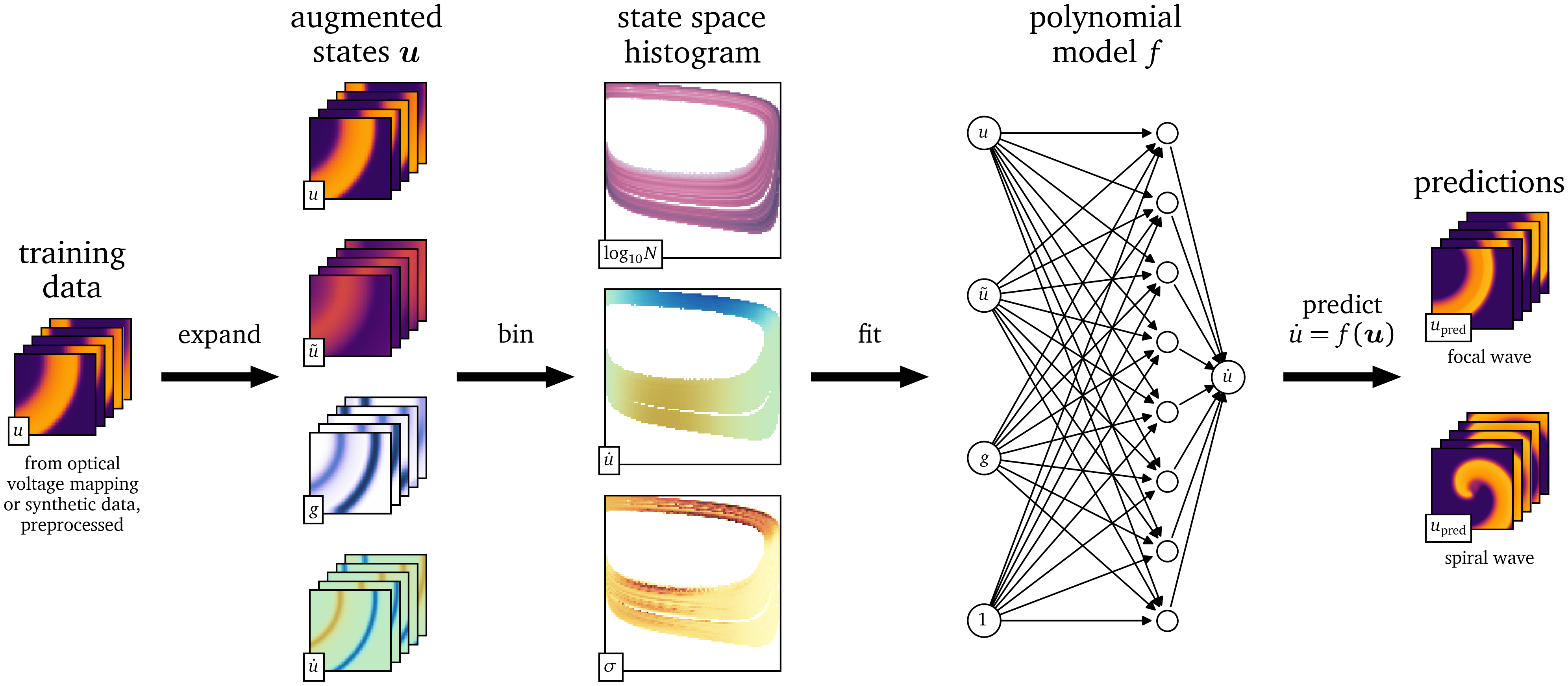
Figure 1: Outline of the model fitting procedure. In the first step, relevant features are extracted from the spatio-temporal data $u$. Then the state space is discretised and histogrammed. The value of the time-derivative $\dot u$ of the main variable is analysed statistically in this state space. A model can then be fit to the state space and used to predict the evolution of the medium.
Methods
Data acquisition
In this work, we study spatio-temporal data from two excitable media: an in-vitro data set from OVM of monolayers of cardiomyogenically differentiated hiAMs and an in-silico data set from finite-differences simulations solving the mono-domain equations (Clayton et al., 2011). In this section, we outline how these data are generated and processed.
Optical voltage mapping
To obtain a two-dimensional recording of the electrical activity of tissue as an in-vitro data set, we performed OVM of hiAM monolayers in 10- wells of six-well culture plates (Harlaar et al., 2022). The recorded data consist of one variable, i.e., the measured difference in intensity of the light emitted by the voltage-sensitive dye, over space and time. We have used a MiCAM05-Ultima camera by SciMedia with a resolution of 100x100 pixels. With the particular configuration of lenses, each square pixel has a size of $\Delta x = {250~\mathrm{{u}{m}}}$. For the recordings, we use the lowest supported duration between frames of $\Delta t = {1~\mathrm{{m}{s}}}$. We record ${61440}$ consecutive frames, which corresponds to slightly more than a minute and lines up nicely in the camera’s file format. For modelling purposes, we assume that the monolayer is approximately homogeneous and isotropic.
To excite the tissue, we place a bi-polar stimulation electrode with two poles with a diameter of and inter-electrode spacing of at the well’s boundary, and stimulate with $N_\text{pulse}=200$ current pulses of random amplitude, random duration, and random timing. We call this procedure the stochastic burst pacing (SBP) protocol, inspired by stochastic pacing experiments done by Krogh-Madsen et al. (2005). The amplitudes $A_n$ are sampled from a uniform distribution $\operatorname{U}{{\left( {-0.8~\mathrm{{m}{A}}}, {0.8~\mathrm{{m}{A}}} \right)}}$. The times $T_n = T_{\text{u}} + T_{\text{e}}$ between subsequent pulses are sampled from a combination of a uniform and exponential distribution: $$ \begin{aligned} T_{\text{u}} &\sim \operatorname{U}{{\left( {0~\mathrm{{m}{s}}}, {50~\mathrm{{m}{s}}} \right)}} \\ T_{\text{e}} &\sim \operatorname{Exp}{{\left( 1/{200~\mathrm{{m}{s}}} \right)}} \end{aligned} \qquad{(1)}$$ where $\operatorname{U}{{\left( a, b \right)}}$ denotes the uniform distribution on the interval ${{\left[ a, b \right]}}$ and $\operatorname{Exp}{{\left( \lambda \right)}}$ the exponential distribution with decay rate $\lambda$: $$ \operatorname{Exp}{{\left( \lambda \right)}}{{\left( t \right)}} \propto \begin{cases} {{\mathrm{e}^{-\lambda t}}} & t \ge 0 \\ 0 & t < 0 \end{cases} \qquad{(2)}$$
We choose this probability distribution of durations such that, on the one hand, it covers a typical range of values, but on the other, occasionally, durations are sampled that are much longer than usual.
The durations $\tau_n = \tau_{\text{u}} + \tau_{\text{e}}$ of stimulation are sampled from a similar probability distribution: $$ \begin{aligned} \tau_{\text{u}} &\sim \operatorname{U}{{\left( {0~\mathrm{{m}{s}}}, {10~\mathrm{{m}{s}}} \right)}} \\ \tau_{\text{e}} &\sim \operatorname{Exp}{{\left( 1/{40~\mathrm{{m}{s}}} \right)}} \end{aligned} \qquad{(3)}$$
The stimulus current then takes the form: $$ I_\text{stim}{{\left( t \right)}} = \sum_{n=1}^{N_\text{pulse}} A_n {{\left[ \operatorname{H}{{\left( t - t_n \right)}} - \operatorname{H}{{\left( t - t_n - \tau_n \right)}} \right]}} \qquad{(4)}$$ with the start time of the $n$-th pulse: $$ t_n = \sum_{m=1}^{n} {{\left[ T_{m} + \tau_{m} \right]}} \qquad{(5)}$$ and the Heaviside function: $$ \operatorname{H}{{\left( t \right)}} = \begin{cases} 0 & t < 0 \\ \frac{1}{2} & t = 0 \\ 1 & t > 0 \end{cases} \qquad{(6)}$$
We preprocess these data in a similar way as in a previous publication (Kabus et al., 2022) by Gaussian blurring with a kernel size of three grid points and rescale the data to zero-mean and unit variance.
To bring the resting state close to zero, we subtract the baseline of the data. As baseline, we take the most common recorded intensity in each 4x4 pixel neighbourhood over a time span of This is based on the assumption that this most common value corresponds to the resting state.
The final preprocessing step for this data set is to smooth the data using an exponential moving average (EMA) with $\alpha = 0.1$, which, for time $t \ge 0$ with frame duration $\Delta t$ and the signal over time $s{{\left( t \right)}}$ at each position in space, is iteratively defined as: $$ \tilde s{{\left( t \right)}} = \begin{cases} \alpha s{{\left( t \right)}} + {{\left[ 1 - \alpha \right]}} \tilde s{{\left( t - \Delta t \right)}} & t > 0 \\ s{{\left( t=0 \right)}} & t = 0 \end{cases} \qquad{(7)}$$ which, within first-order time discretisation, is equivalent to: $$ \tilde s{{\left( t \right)}} = {{\mathrm{e}^{-a t}}} s{{\left( 0 \right)}} + a \int_0^t {{\mathrm{e}^{a {{\left[ t' - t \right]}}}}} s{{\left( t' \right)}} \;\mathrm{d} t' \qquad{(8)}$$ with $a = \frac{\alpha}{\Delta t} > 0$.
We refer to this recording as the OVM data set and $u{{\left( t, {{\bm{{x}}}} \right)}}$ denotes the unit-less signal after preprocessing scaled such that the resting state is close to $u=0$ and the excited state around $u=1$. This signal $u$ corresponds to the electrical activity of the cells, i.e., it is linked to the transmembrane voltage over space and time.
Only for qualitative comparisons after a data-driven model is fit to the OVM data set, a second OVM recording is used. In this second recording, several minutes after rotor formation through burst pacing, the resulting single, stable spiral wave is observed. This experiment is also performed with hiAMs in the same six-well format as before and at the same spatial resolution but at a lower temporal resolution of between frames. We preprocess these data in the same way as the main OVM data set.
Numerical simulation
To obtain a fully controllable testing data set, we ran an in-silico experiment similar to the in-vitro experiment in section 2.1.1. We use the finite-differences method to solve the reaction-diffusion system using a rescaled version of the minimalist two-variable tissue model by Aliev & Panfilov (1996), or in short the AP96 model, whose equations we will briefly summarise (Eq. 11).
As the diffusivity is proportional to the square of the CV, we set it such that the medium has a measured CV close to that of hiAMs (Clayton et al., 2011; Harlaar et al., 2022): $$ \begin{aligned} D &= {0.0625~\mathrm{{m}{m}{^2}{/}{m}{s}}} \\ \Rightarrow \text{CV} &= {0.17~\mathrm{{m}{/}{s}}} \end{aligned} \qquad{(9)}$$ We rescale the entire model over time such that its APD has a value of roughly the APD of hiAMs (Harlaar et al., 2022): $$ r = \frac{\text{APD}_\text{AP96}}{\text{APD}_\text{hiAM}} = \frac{{25.58}}{{100~\mathrm{{m}{s}}}} = {0.2558~\mathrm{\frac{1}{{m}{s}}}} \qquad{(10)}$$
The time derivatives are rescaled by this time scaling factor $r$ (Aliev & Panfilov, 1996): $$ \begin{aligned} \partial_t u &= \nabla \cdot D \nabla u - r k u {{\left[ u - a \right]}} {{\left[ u - 1 \right]}} - r u v + \frac{i_\text{stim}}{C} \\ \partial_t v &= - r \epsilon v - r \epsilon k u {{\left[ u - a - 1 \right]}} \\ \epsilon &= \epsilon_0 + \frac{\mu_1 v}{u + \mu_2} \end{aligned} \qquad{(11)}$$
By doing so, we introduced the millimetre as the spatial unit and the millisecond for time into the AP96 model, which uses arbitrary space and time units. The variables $u{{\left( t, {{\bm{{x}}}} \right)}}$ and $v{{\left( t, {{\bm{{x}}}} \right)}}$ remain unit-less. The value $u=0$ corresponds to the resting state and when excited, $u$ approaches the value $u=1$.
For all other parameters, $a$, $\epsilon_0$, $k$, $\mu_1$, and $\mu_2$, which are all unitless, we use the default values, as in the original publication by Aliev & Panfilov (1996). An overview of all parameters can be found in Table 1.
| Parameter | Value |
|---|---|
| $a$ | 0.15 |
| $\epsilon_0$ | 0.002 |
| $k$ | 8 |
| $\mu_1$ | 0.2 |
| $\mu_2$ | 0.3 |
| $D$ | |
| $r$ | ${0.2558~\mathrm{{m}{s}}}$ |
Table 1: Parameters of the rescaled AP96 model.
We have run a simulation over ${43104}$ frames at $\Delta t = {1~\mathrm{{m}{s}}}$ per frame at the same resolution as for the in-vitro OVM data and with the same SBP protocol. The length of the simulation was chosen such that the tissue can fully recover after the last of the 200 pulses of the SBP protocol. The electrode was placed off-centre at the side of one edge of the medium. For the time integration, we used a simple forward Euler step with numerical time step ${0.1~\mathrm{{m}{s}}}$ and a second-order central finite-differences five-point stencil for the Laplacian $\nabla \cdot D \nabla$. The square simulated tissue was homogeneous and isotropic with no-flux boundary conditions.
We refer to this synthetic recording as the AP96 data set. We only include the variable $u{{\left( t, {{\bm{{x}}}} \right)}}$ in the data set, as in the in-vitro data set, i.e., the OVM data set. For surrogate model fitting, we hence also only use one variable related to the transmembrane voltage of the tissue and not the internal state of the cell, which in the AP96 model is encapsulated in the second variable $v{{\left( t, {{\bm{{x}}}} \right)}}$.
In the subsequent steps, only these data will be used, partially as training data and partially as testing data. However, we also generate auxiliary data sets for the AP96 model that are only used for qualitative comparisons with the data-driven models after fitting.
To generate a recording of a rotor using the AP96 model, we ran another two-dimensional simulation at the same resolution in space and time with initial conditions that led to a spiral wave: The transmembrane voltage was set to a value of $u = {0.95}$ within the rectangle ${{\left[ 0, {0.5}L_x \right]}}\times{{\left[ {0.3}L_y, {0.5}L_y \right]}}$, and the second variable to $v = 1$ within a second rectangle ${{\left[ 0, {0.5}L_x \right]}}\times{{\left[ {0.4}L_y, {0.6}L_y \right]}}$, where $L_x = L_y = {100~\mathrm{{m}{m}}}$. Gaussian blurring with a radius of four grid lengths was applied to avoid steep gradients at the edge of the rectangles.
We also measured restitution curves, i.e., APD and CV as functions of the cycle length (CL) of stimulation. For this, we ran a one-dimensional cable simulation of the model with the same spatial and temporal resolution. At the left end of the cable, we stimulated by instantaneously setting $u$ to a value above the excitation threshold to trigger a wave travelling to the right. We repeatedly stimulated starting at a CL of decreasing in steps of until we reached a CL where not every stimulus resulted in a pulse that traveled through the entire cable, i.e., where 2:1 conduction block begins.
State space augmentation
The multi-dimensional space spanned by all variables describing the state of the modelled medium, ${{\bm{{u}}}} = {{{{\left[ u, v, ... \right]}}}^\mathrm{T}}$, is called state space in contrast to the physical space spanned by ${{\bm{{x}}}}$ and time $t$.
An in-silico tissue model usually prescribes a unique reaction ${{\bm{{R}}}}$ at each position ${{\bm{{u}}}}$ in the state space. We write a more generic version of Eq. 11, the mono-domain description (Clayton et al., 2011): $$ \begin{aligned} \partial_t {{\bm{{u}}}} &= {{\bm{{P}}}} \nabla \cdot {{\bm{{D}}}} \nabla {{\bm{{u}}}} + {{\bm{{R}}}} {{\left( {{\bm{{u}}}} \right)}} \end{aligned} \qquad{(12)}$$ with the diffusivity matrix ${{\bm{{D}}}}$, where ${{\bm{{P}}}}$ is a diagonal matrix describing which variables in ${{\bm{{u}}}}$ are to be diffused.
For the two-variable AP96 model, with ${{\bm{{u}}}} = {{{{\left[ u, v \right]}}}^\mathrm{T}}$ and ${{\bm{{P}}}} = \operatorname{diag}{{\left( 1, 0 \right)}}$, the state space of the AP96 model is shown in Fig. 2, coloured only by the component in $u$ of the reaction term ${{\bm{{R}}}}$. It can be seen that the second variable $v$ can be used to distinguish cases with positive and negative reaction at the same value of $u$. A model that can describe both excitation from a resting state and recovery to it, is only possible with at least two variables, such that the inertial manifold can be a loop in the state space.
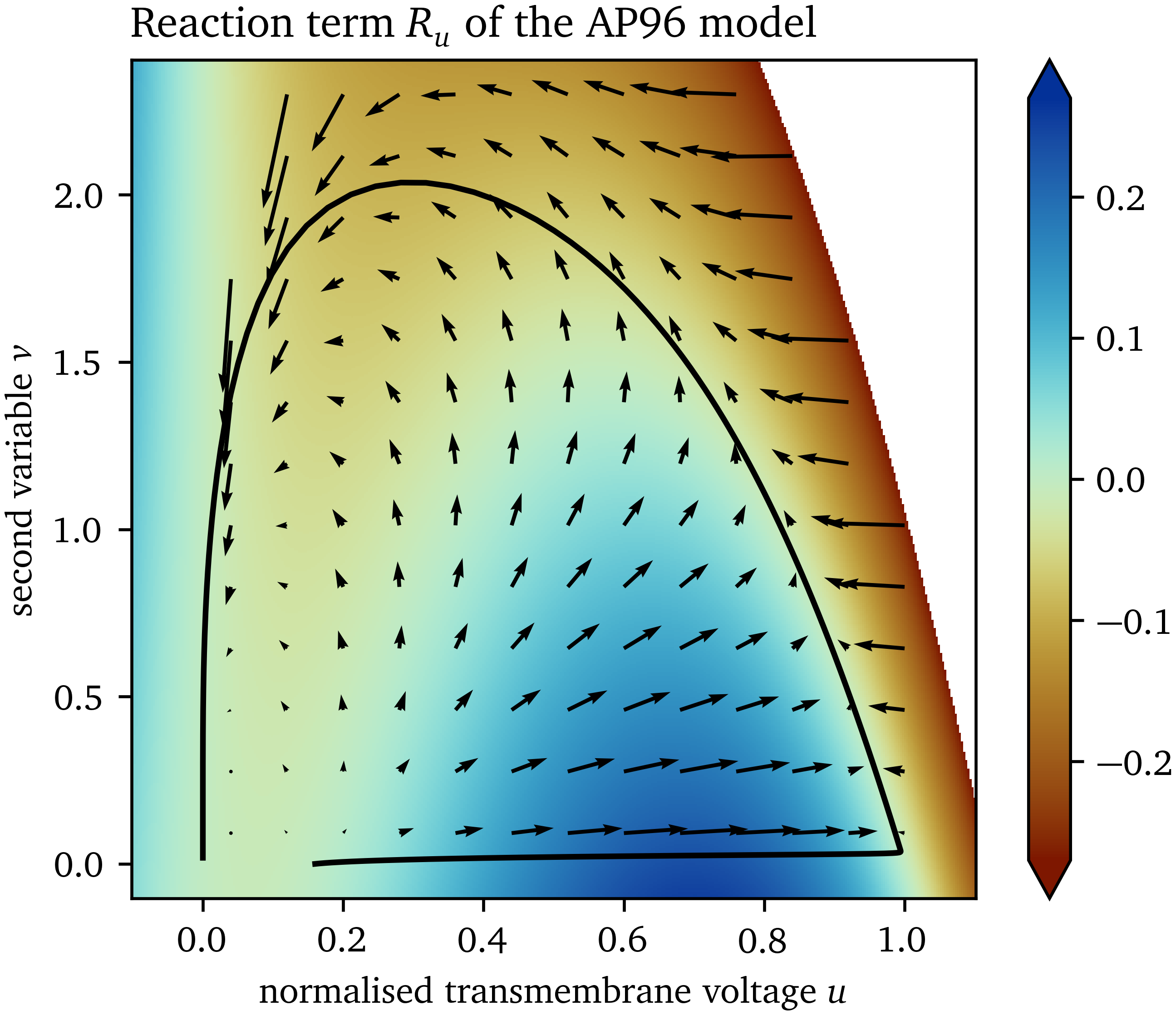
Figure 2: Reaction in state space of the AP96 model. The reaction term ${{\bm{{R}}}}$ is a vector field defining a reaction at each point ${{\bm{{u}}}}$ in the state space. Colouring is according to the $u$-component of the reaction term $R_u$. The trajectory through the state space from excitation of one point is shown as an example.
In both types of data sets considered in this work, we only have data for one variable available, namely $u$. To still be able to differentiate between excitation and recovery, we extract additional information from $u$ over space and time to use as additional states for the state space, so-called augmentations. A well-designed augmented state space unfolds the data such that cells in the tissue with different histories are identified by different augmented state vectors.
As we want to find models that can be used as forward models in a similar way as in Eq. 12, we impose two more requirements on the states with which we augment the state space:
- Augmentations should be local in space, i.e., they should only use states within a neighbourhood around each point.
- Causality must be respected, i.e., only data from previous points in time and the current point in time may be used to compute each augmentation.
The two augmentations that we found to be most useful for model creation are presented in the remainder of this section.
Exponential moving averages
The goal of the state space augmentation is to capture that the model can evolve differently from the same value of $u$. This value may increase at the front of waves, during excitation, or decrease at the wave backs, during recovery.
One way to sense excitation and recovery is by expanding the state space with augmented states that capture the passage of time. A naïve way to do so may be to just include a time-delayed signal, which is a useful augmentation in phase mapping (Gray et al., 1995). This is, however, not very robust to noise, as noise in the past may directly impact the present. Another option may be to use Hilbert transforms, but as their computation involves an integral over all of time, they violate causality and are therefore not meeting our requirements (Kuklik et al., 2014).
The EMA (Eq. 7) is robust to noise and typically lags behind the signal by an amount of time inversely proportional to the constant $\alpha$. It can intuitively be used to differentiate between excitation and recovery for signals $u$ in-between the resting state and excited state: If an EMA with a suitable scale $\alpha$ is lower than $u$, it is likely that the medium is currently getting excited; if it is higher, the cells are likely recovering.
Multiple EMAs can be used to be able to capture more advanced behaviour: With an appropriately chosen $\alpha$, we can differentiate between states where the tissue is activated a lot and where it is mostly resting. With such an EMA, restitution characteristics can be captured.
Here, we augment the AP96 data with a single EMA $\tilde u$ with $\alpha = {0.03}$. For $\tilde u$ in the OVM data, we use $\alpha = {0.008}$.
Standard deviation as a proxy for the absolute gradient
We also conjecture that information about the slopes and higher derivatives in space of $u$ is useful for a well fitting data-driven model. In the reaction-diffusion description, the Laplacian is used to capture curvature effects in space. Because it is a second-order derivative, it is very sensitive to noise. The absolute value of the gradient in combination with other state space variables can also encode much information about the slopes of $u$. We use a proxy for the absolute gradient in a neighbourhood with high robustness with respect to noise. Such a proxy is the standard deviation (SD) of the signal $u$ in the local neighbourhood up to a radius $R$ around ${{\bm{{x}}}}$.
It can be shown analytically that the SD is proportional to the absolute gradient of a plane $h{{\left( {{\bm{{x}}}} \right)}} = {{{{\bm{{w}}}}}^\mathrm{T}} {{\bm{{x}}}} + b$, which evaluates to ${{\left\lVert \nabla h \right\rVert}} = {{\left\lVert {{\bm{{w}}}} \right\rVert}}$. The SD in a spherical neighbourhood $\mathcal N$ up to a radius $R$ around the origin can be found via integration in polar coordinates $r$, ${\varphi}$: $$ \begin{aligned} \sigma_h^2 &= {{\left\langle {{\left[ h-b \right]}}^2 \right\rangle}} = \frac {1}{\int_{\mathcal N} \mathrm{d} {{\bm{{x}}}}\;} \int_{\mathcal N} \mathrm{d} {{\bm{{x}}}}\; {{\left[ {{{{\bm{{w}}}}}^\mathrm{T}} {{\bm{{x}}}} \right]}}^2 \\ \sigma_h^2 &= \frac {1}{\pi R^2} \int_{0}^{R} \mathrm{d} r\; \int_{0}^{2\pi} \mathrm{d} {\varphi}\; {{\left[ w_x r\cos{\varphi}+ w_y r\sin{\varphi}\right]}}^2 \\ \sigma_h &= \frac {R}{2} {{\left\lVert {{\bm{{w}}}} \right\rVert}} \end{aligned} \qquad{(13)}$$ Analogously, a similar relation can be shown in three dimensions: $$ \sigma_h = \frac{R}{\sqrt{5}} {{\left\lVert {{\bm{{w}}}} \right\rVert}} \qquad{(14)}$$
Assuming that the signal $u$ varies slow enough that a linear function can approximate it well within the chosen neighbourhood, the SD can be used to compute its absolute gradient. Despite the relatively high time-derivative $\dot u$ of the cardiac action potential during its upstroke, and hence $\nabla u$, we can make this assumption if the resolution is sufficiently high.
Note that the SD has the useful property, that it can still be computed at or near the boundary of the medium, just based on fewer samples than for fully interior points.
To capture gradient information, we augment the AP96 data set with an SD variable for the neighbourhood up to a radius $R = 5 \Delta x$ around each point ${{\bm{{x}}}}$ and denote it by $g$. For $g$ in the OVM data set, we use a larger neighbourhood with $R = 8 \Delta x$ for the SD calculation.
State space histograms
In the usual dynamics of the excitable systems we study in this work, not all points ${{\bm{{u}}}}$ in the state space are equally likely. Some state vectors ${{\bm{{u}}}}$ may be quite common as being part of the inertial manifold, while others might be completely absent in the data.
For example, for the AP96 model with ${{\bm{{u}}}} = {{{{\left[ u, v \right]}}}^\mathrm{T}}$, it can be seen in Fig. 3 that a part of the state space is not visited and most of the samples are on the inertial manifold, a closed approximately one-dimensional loop. We conjecture that in higher dimensions the state space is even more sparse, e.g. in case of detailed ionic models, some of which contain more than ten state variables.
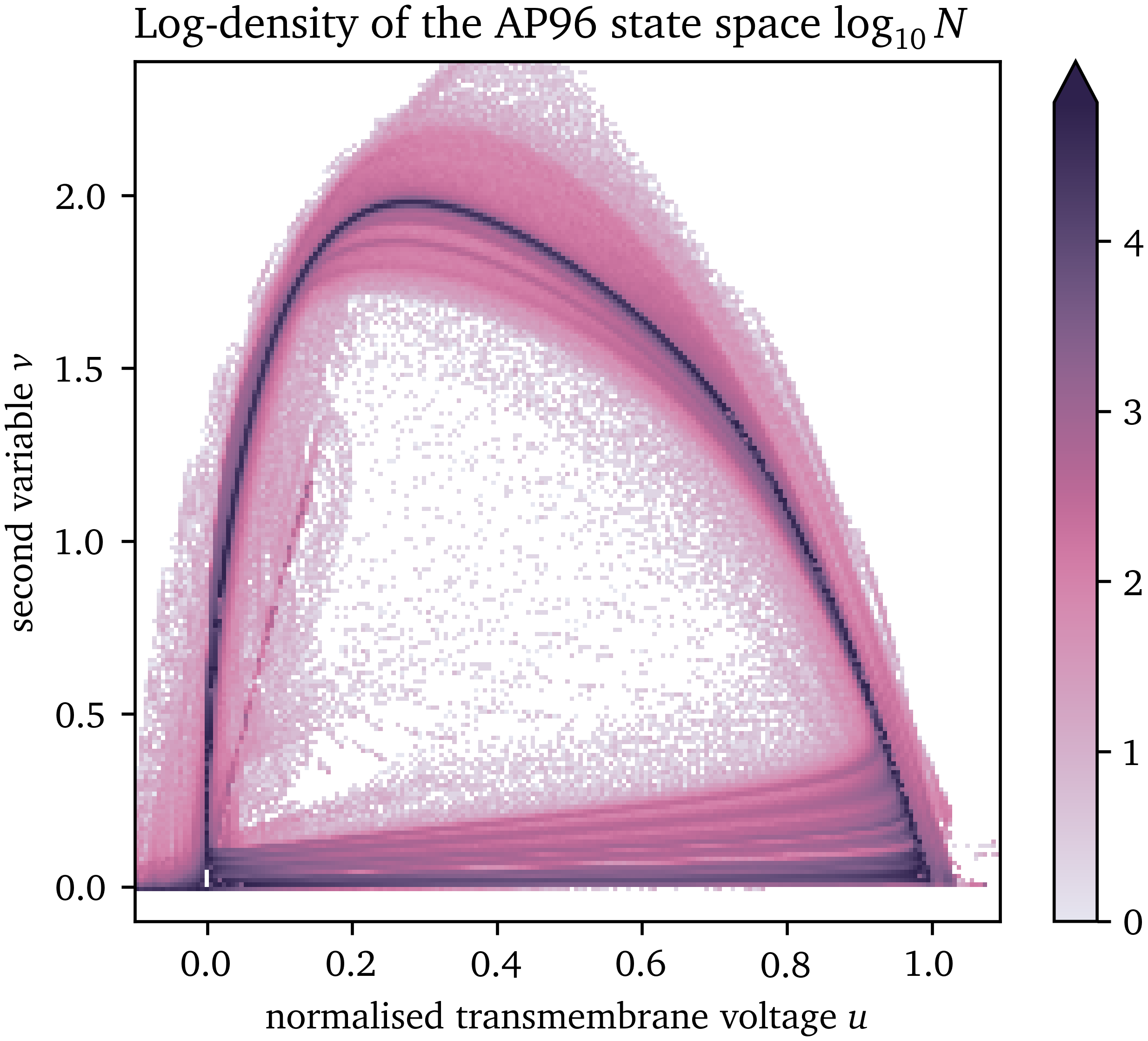
Figure 3: Likelihood of each point in the state space of the AP96 model for the numerical simulation generating the data set used for surrogate model fitting.
With the chosen state space expansion (section 2.2), the state vector is ${{\bm{{u}}}} = {{{{\left[ u, \tilde u, g \right]}}}^\mathrm{T}}$. We discretise the state space to 100 bins in each dimension and collect the data in a multi-dimensional histogram. This results in three-dimensional state space histograms for the two data sets with ${10}^6$ bins each. For efficient memory usage, these histograms are computationally implemented using multi-dimensional sparse arrays. Regions in the state space containing no data do not take up memory in this way. We can then fit the models to the average value inside each bin instead of to all data points. This efficient memory management enables building even higher-dimensional state spaces, though in this work we require only three variables.
The time-derivative $\dot u$ fully defines the reaction of the data-driven models developed in this work. The reason for this is that all other variables in the state vector ${{\bm{{u}}}}$ can be derived from the one variable $u$ over space and time.
In a well chosen state space, for each state vector ${{\bm{{u}}}}$, the reaction $\dot u$ is the same, i.e., the states are well separated. Therefore, we calculate the mean value of $\dot u$ computed using finite-differences at each bin in the discretised state space, as well as its SD. This mean value of $\dot u$ takes a similar role as $R_u$ for the AP96 model and “colours” the state space in a comparable way to $R_u$ in Fig. 2.
Model fitting
A data-driven model will be fit to the data in state space as a scalar-valued function $f$: $$ f : {{\bm{{u}}}} \mapsto \dot u \qquad{(15)}$$ such that the model consists of the state space expansion ${{\bm{{u}}}}$ by calculating the EMA (Eq. 7), the SD within the neighbourhoods around each point (section 2.2.2), as well as the forward Euler step: $$ u{{\left( t+\Delta t, {{\bm{{x}}}} \right)}} = u{{\left( t, {{\bm{{x}}}} \right)}} + \Delta t f{{\left( {{\bm{{u}}}}{{\left( t, {{\bm{{x}}}} \right)}} \right)}} \qquad{(16)}$$
As the model function $f$, we choose a low-order polynomial which is linear with respect to each of the components: $$ f{\left({{\bm{{u}}}}\right)} = w_{\tilde{u} g u} \tilde{u} g u + w_{\tilde{u} g} \tilde{u} g + w_{\tilde{u} u} \tilde{u} u + w_{\tilde{u}} \tilde{u} + w_{g u} g u + w_{g} g + w_{u} u + w \qquad{(17)}$$
Assuming that the SD $g$ approximates the absolute gradient ${{\left\lVert \nabla u \right\rVert}}$ of the main state variable $u$ well, we hence essentially describe the propagation of the activation waves using advection, instead of diffusion (Eq. 12): $$\begin{aligned} \partial_t u &= f{{\left( {{\bm{{u}}}} \right)}} = f_0{{\left( u, \tilde u \right)}} + c_1 f_1{{\left( u, \tilde u \right)}} {{\left\lVert \nabla u \right\rVert}} \\ f_0{{\left( u, \tilde u \right)}} &= w + w_u u + w_{\tilde u} \tilde u + w_{\tilde u u} \tilde u u \\ f_1{{\left( u, \tilde u \right)}} &= w_{g} + w_{g u} u + w_{\tilde u g} \tilde u + w_{\tilde u g u} \tilde u u \\ \tilde u{{\left( t \right)}} &= {{\mathrm{e}^{-a t}}} u{{\left( 0 \right)}} + a \int_0^t {{\mathrm{e}^{a {{\left[ t' - t \right]}}}}} u{{\left( t' \right)}} \;\mathrm{d} t' \end{aligned}\qquad{(18)}$$ with real-valued scalar constants $a, c_1, w_{...}$ and $g \approx c_1 {{\left\lVert \nabla u \right\rVert}}$. For an appropriate choice of parameters, obtained for instance through fitting, Eq. 18 describe a model of excitation in an advection-regression framework.
To prevent the fit model from leaving the valid state space, after each forward Euler step, we clip the predicted $u$ to the range ${{\left[ u_{\min},u_{\max} \right]}}$ for which we have training data, the so-called valid range. Note that this also limits the EMA $\tilde u$ to that range, while the SD $g$ can still leave the range observed in the data, i.e., for larger than typical slopes.
In each step forward in time, $t \leftarrow t + \Delta t$, we update the state vector ${{\bm{{u}}}} = {{{{\left[ u, \tilde u, g \right]}}}^\mathrm{T}}$ of the data-driven model according to the following pseudocode:
- Compute the new value of $u$ at each point ${{\bm{{x}}}}$ using the polynomial $f$ (Eq. 16; Eq. 17): $$ \begin{aligned} &u \leftarrow u + \Delta t f{{\left( {{\bm{{u}}}} \right)}} \\ &u \leftarrow \max{{\left( u_{\min}, \min{{\left( u, u_{\max} \right)}} \right)}} \end{aligned} \qquad{(19)}$$
- Update the EMA $\tilde u$ based on its old value and the updated $u$ (Eq. 7): $$ \tilde u \leftarrow \alpha u + {{\left[ 1 - \alpha \right]}} \, \tilde u \qquad{(20)}$$
- Calculate the SD $g$ of the updated $u$ (section 2.2.2): $$ g \leftarrow {{\left\langle u^2 - {{\left\langle u \right\rangle}}^2 \right\rangle}}^{\frac{1}{2}} \qquad{(21)}$$ where ${{\left\langle \bullet \right\rangle}}$ denotes the average of all points in the spherical neighbourhood $\mathcal N$ of each position ${{\bm{{x}}}}$ up to a radius $R$.
To find the optimal model function $f$, we use the least-squares algorithm to find the polynomial of the given order which minimises the loss: $$ \mathcal L{{\left( f \right)}} = \sum_{{{\bm{{u}}}} \in \mathcal U} N{{\left( {{\bm{{u}}}} \right)}} {{\left[ \dot u{{\left( {{\bm{{u}}}} \right)}} - f{{\left( {{\bm{{u}}}} \right)}} \right]}}^2 + \sum_{{{\bm{{u}}}} \in \mathcal R} f^2{{\left( {{\bm{{u}}}} \right)}} \qquad{(22)}$$
where $\mathcal U$ denotes the centres of all bins in the discretised state space containing at least one sample, i.e., one data point, and $N{{\left( {{\bm{{u}}}} \right)}}$ is the number of samples in the bin ${{\bm{{u}}}}$. To regularise the model space in favour of more physically realistic models, we add additional co-location points $\mathcal R$ outside of $\mathcal U$ at which we assume $f$ should be close to zero. We choose these co-location points $\mathcal R$ by Latin hypercube sampling and only keep points for which no data is contained in the data set $\mathcal U$ (McKay et al., 2000). We choose the number $N_{\mathcal R}$ of co-location points $\mathcal R$ based on the number $N_{\mathcal U}$ of non-empty bins in the data set $\mathcal U$: $$ N_{\mathcal R} = {0.5} \, N_{\mathcal U} \qquad{(23)}$$
As training data spanning the state space $\mathcal U$ that the model is fit to, we use all frames up to just before the last pulse of the SBP in each recording. The frames of the last pulse of each recording are then used as testing data, i.e., as a reference to compare with the predicted frames of the data-driven model. We only include points at least 20 grid points away from the boundary to minimise boundary effects on the used data.
Besides this first simulation that can be directly and quantitatively compared to the reference for both data sets, we also run simulations using the data-driven models to compare them qualitatively with the reference model, i.e., the AP96 model for the synthetic data set, and the in-vitro model for the OVM data. As the second simulation, for both data-driven models, we run a similar rectangle-based protocol to the one used to stimulate spirals for the reference AP96 model (section 2.1.2). Here, we use the same stimulation values for $u$, but $\tilde u = 0.6$ inside the second rectangle and $\tilde u = 0.1$ outside of it. Thirdly, we also run a one-dimensional cable simulation to obtain APD and CV restitution curves for the fit surrogate AP96 model with the same restitution stimulation protocol as outlined for the reference AP96 model in section 2.1.2
Results
In this section, we present how the state space expansion and data-driven models as described in section 2, deal with the two data sets. Since the results for the in-silico synthetic data are easier to interpret, we begin with those data.
Surrogate model for synthetic data
State space
For the data set from numerical simulation of the AP96 model (cf. section 2.1.2), the three-dimensional state space spanned by ${{\bm{{u}}}} = {{{{\left[ u, \tilde u, g \right]}}}^\mathrm{T}}$ is quite sparse. ${95695}$ bins in this space contain at least one data point, which corresponds to ${9~\mathrm{\%}}$ of all bins. Of these bins, ${40~\mathrm{\%}}$ contain at least 10 data points. Non-empty bins contain ${230}$ data points on average.
In Fig. 4, we present a three-dimensional view of the state space and two different two-dimensional projections of the state space; to $u$ and $g$, and to $u$ and $\tilde u$, respectively. Panel A shows that most data points lay on a loop-like inertial manifold, while a large volume of the state space is still covered by data points (panel B). Colouring by the mean of $\dot u$, we can see that the two halves of the loop nicely distinguish between excitation and recovery, see the blue and red shades in panel C. Note that the colouring of the state space in panel D corresponds to the SD $\sigma$ and not to the SD $g$. To be more specific, this panel is coloured by the SD $\sigma$ of the samples of the time-derivative $\dot u$ in the bins, instead of the SD $g$ of the signal $u$ in the neighbourhoods around each point ${{\bm{{x}}}}$, which is one of the axes spanning the state space in Fig. 4. In large parts of these projections, the SD $\sigma$ is much lower than the mean absolute value of $\dot u$, showing that the model’s possible states are well-separated in the chosen state space ${{\bm{{u}}}}$.
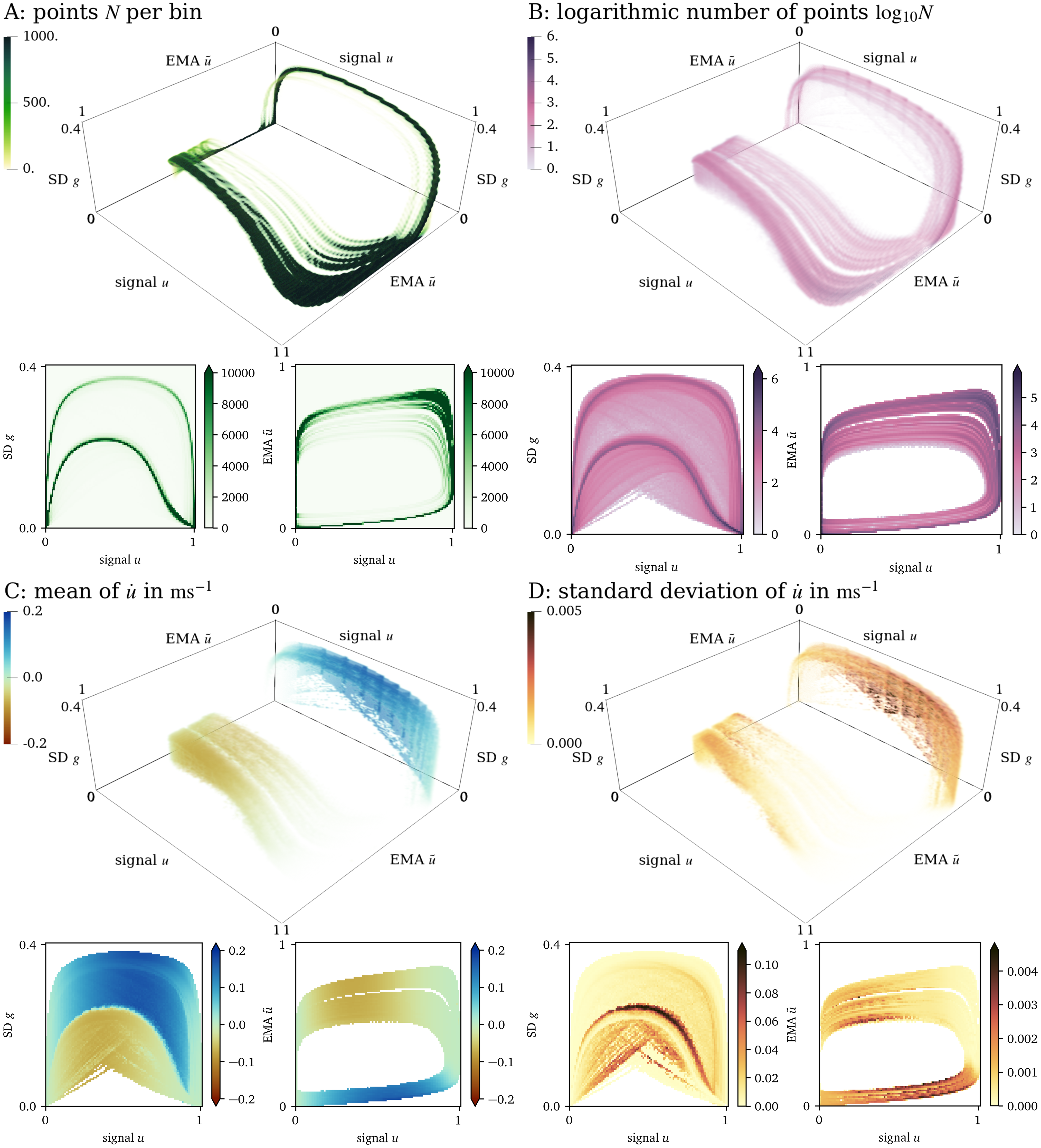
Figure 4: Visualisation of the three-dimensional state space for the AP96 data set and projections onto two dimensions. (A): By colouring the space by the number $N$ of points in each bin, it can be seen that most points lay on a loop. (B): Colouring by $\log_{10}{N}$, we can see that still a large volume of the space is covered by data. (C): Looking at the mean of $\dot u$ at each bin in this projection, we can see that in one side of the loop, $u$ increases while it decreases at the other side. (D): The standard deviation of $\dot u$ is indicative of whether the states have been chosen well.
Forward model
A model in the context of this work consists of a “colouring” of the entire three-dimensional state space representing the $\dot u$ at each possible state ${{\bm{{u}}}}$.
The data-driven surrogate model $f$ is fit to the three-dimensional state space as outlined in section 2.4 resulting in: $$ \begin{aligned} f{\left({{\bm{{u}}}}\right)} =& - {0.22407}\, \tilde{u} g u - {0.82589}\, \tilde{u} g + {0.0054601}\, \tilde{u} u + {0.021655}\, \tilde{u} \\& + {0.31082}\, g u + {0.23077}\, g - {0.0081478}\, u - {0.0097110} \end{aligned} \qquad{(24)}$$
Subsequently, a forward simulation is performed with the model, leading to a prediction of $u$ based on the history until that point which can be compared to the reference evolution of $u$ in Fig. 5. This simple model displays excitation and recovery, as well as propagation of the wave. The predicted evolution is similar to its reference: The values for the plateau-phase and resting state are close to the reference values. The depolarisation at the wave front is a bit too late, leading to predicted values that are too low. Likewise, the repolarisation at the wave back is too late, such that there the predicted values are too high.
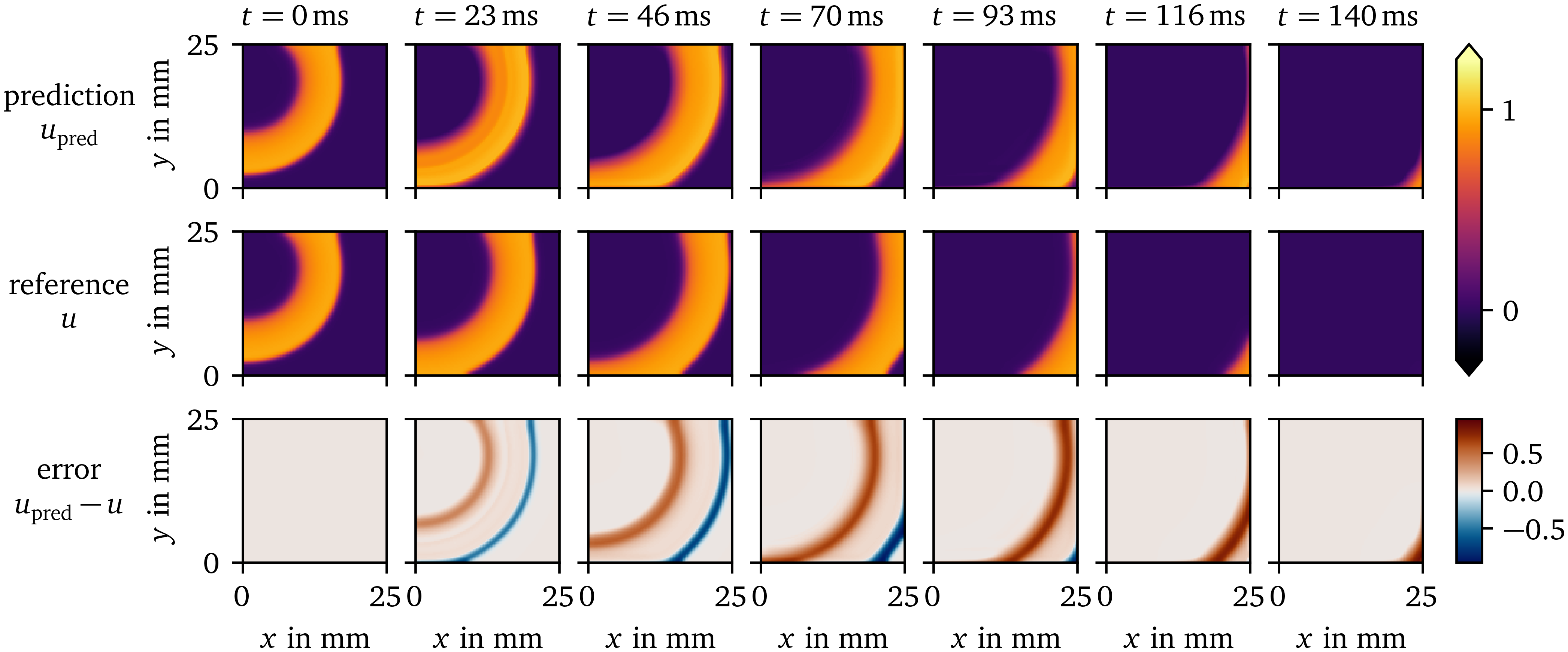
Figure 5: Prediction of the surrogate model over time compared to the reference solution for the AP96 data set. The difference between the prediction and reference is displayed in the bottom row.
Using the method by Bayly et al. (1998), CV has been measured to be ${(0.1403\ ±\ 0.0036)~\mathrm{{m}{/}{s}}}$ for the prediction, and ${(0.1621\ ±\ 0.0065)~\mathrm{{m}{/}{s}}}$ for the reference. This lower propagation velocity leads to the observed delay of wave front and back.
We also computed the average APD of the activity in the central 60x60 pixels of the frame with the polarisation threshold of $u = 0.5$: For the prediction, we measure an APD of ${(56.68\ ±\ 0.48)~\mathrm{{m}{s}}}$, which is slightly longer than the reference of ${(47.25\ ±\ 0.44)~\mathrm{{m}{s}}}$.
At the boundary of the domain, the method is still able to compute the evolution well despite less neighbouring data points being used for the calculation of the SD $g$.
Prediction of a spiral wave
Using similar initial conditions for the data-driven surrogate AP96 model and its reference, we have run simulations leading to spiral waves. In Fig. 6, the resulting evolutions of $u$ over space and time are juxtaposed. It can be seen that the overall wave dynamics are similar, despite the data-driven model only being fit to data from SBP focal waves, i.e., spherical waves growing from a small source region with different timing and amplitudes. The surrogate model predicts wave fronts and backs at similar scales as the reference. The timing of the predicted spiral is also similar to the reference. However, the prediction differs from the reference in the APD of the initial rotation, at the rotor core, and in memory effects. Such a memory effect can clearly be seen in the reference at $t={150~\mathrm{{m}{s}}}$: The recovery to the resting state is much faster in the rectangle where the second variable $v$ of the reference model has been set to a higher value in the initial state of the simulation. This causes a slightly different evolution afterwards.
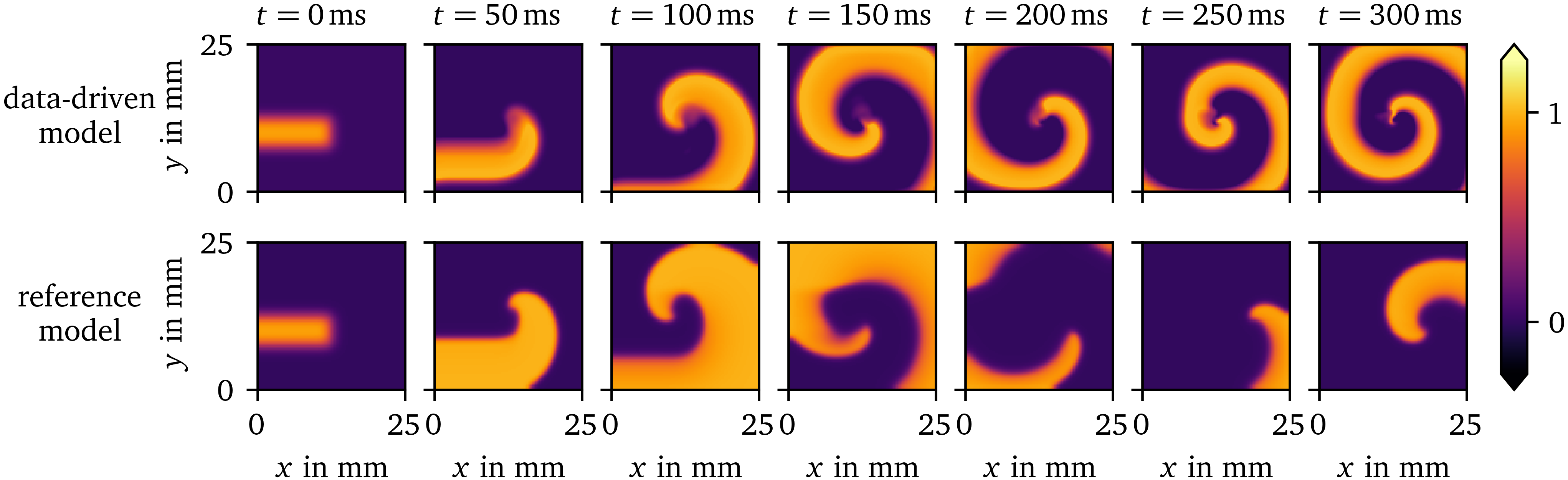
Figure 6: Spiral wave resulting from similar initial conditions for the data-driven surrogate model for the AP96 data set compared to its reference model. The data-driven model can predict the shape of the spiral wave despite only focal waves being included in the training data it is fit to.
Restitution curves
We have also performed one-dimensional cable simulations with the same stimulation protocol for the data-driven surrogate model compared to the rescaled AP96 model for reference. In Fig. 7, the resulting restitution curves of CV (panel A) and APD (panel B) as functions of the CL are shown. The overall shape of the curves for the low-order surrogate model is similar to the reference. However, the predicted CVs are lower than the reference values.
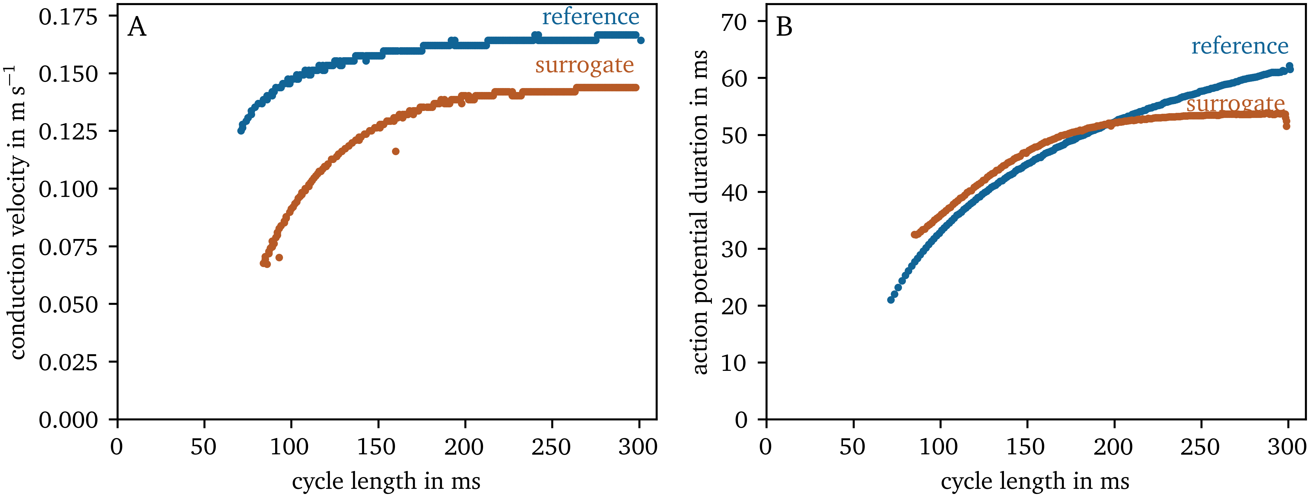
Figure 7: CV and APD restitution curves for the reference AP96 model and its data-driven surrogate model.
Data-driven model for optical mapping data
State space
For the OVM data set of hiAMs (cf. section 2.1.1), the three-dimensional state space spanned by ${{\bm{{u}}}} = {{{{\left[ u, \tilde u, g \right]}}}^\mathrm{T}}$ is also sparse: ${152417}$ bins in this space contain at least one data point, which corresponds to just ${15~\mathrm{\%}}$ of all bins. Of these bins, ${71~\mathrm{\%}}$ contain at least 10 data points. Non-empty bins on average contain ${949}$ data points.
As can be seen in Fig. 8, for these data, we are also observing a loop-like inertial manifold with two halves as in the other data set.
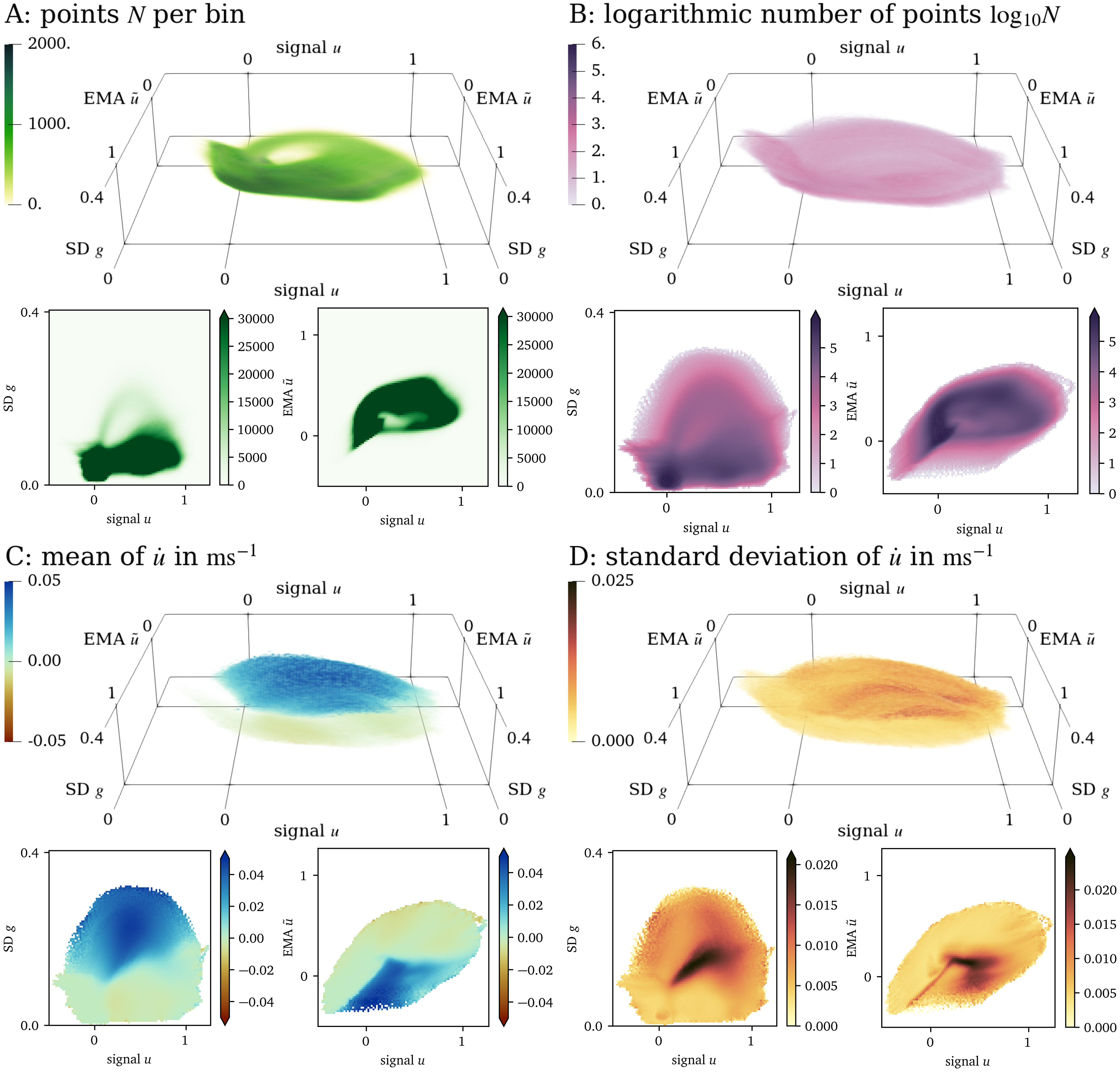
Figure 8: Visualisation of the three-dimensional state space for the OVM data set and projections onto two dimensions in the same style as in Fig. 4.
Forward model
For the OVM data set, the fit polynomial for the data-driven model is: $$ \begin{aligned} f{\left({{\bm{{u}}}}\right)} =& - {0.41392}\, \tilde{u} g u - {0.31842}\, \tilde{u} g + {0.026308}\, \tilde{u} u + {0.0010949}\, \tilde{u} \\& + {0.19341}\, g u + {0.15352}\, g - {0.014174}\, u - {0.0044818} \end{aligned} \qquad{(25)}$$
The prediction by the forward model for the OVM data set is depicted in Fig. 9. It models the overall behaviour of the tissue, i.e., excitation, recovery, and wave propagation, at similar time scales: The APD for an excitation threshold of $u=0.5$ of ${(140.1\ ±\ 5.1)~\mathrm{{m}{s}}}$ for the prediction is longer than the APD of ${(127\ ±\ 36)~\mathrm{{m}{s}}}$ measured for the reference. The CV for the prediction is measured at ${(0.148\ ±\ 0.012)~\mathrm{{m}{/}{s}}}$, and at ${(0.21\ ±\ 0.13)~\mathrm{{m}{/}{s}}}$ for the reference. The large uncertainty in the APD and CV measurements for the reference data is due to small regions of inhomogeneity in the recording. Due to the uncertainty and disparity in APD and CV values between prediction and reference, no reliable restitution curves can been measured for this model.
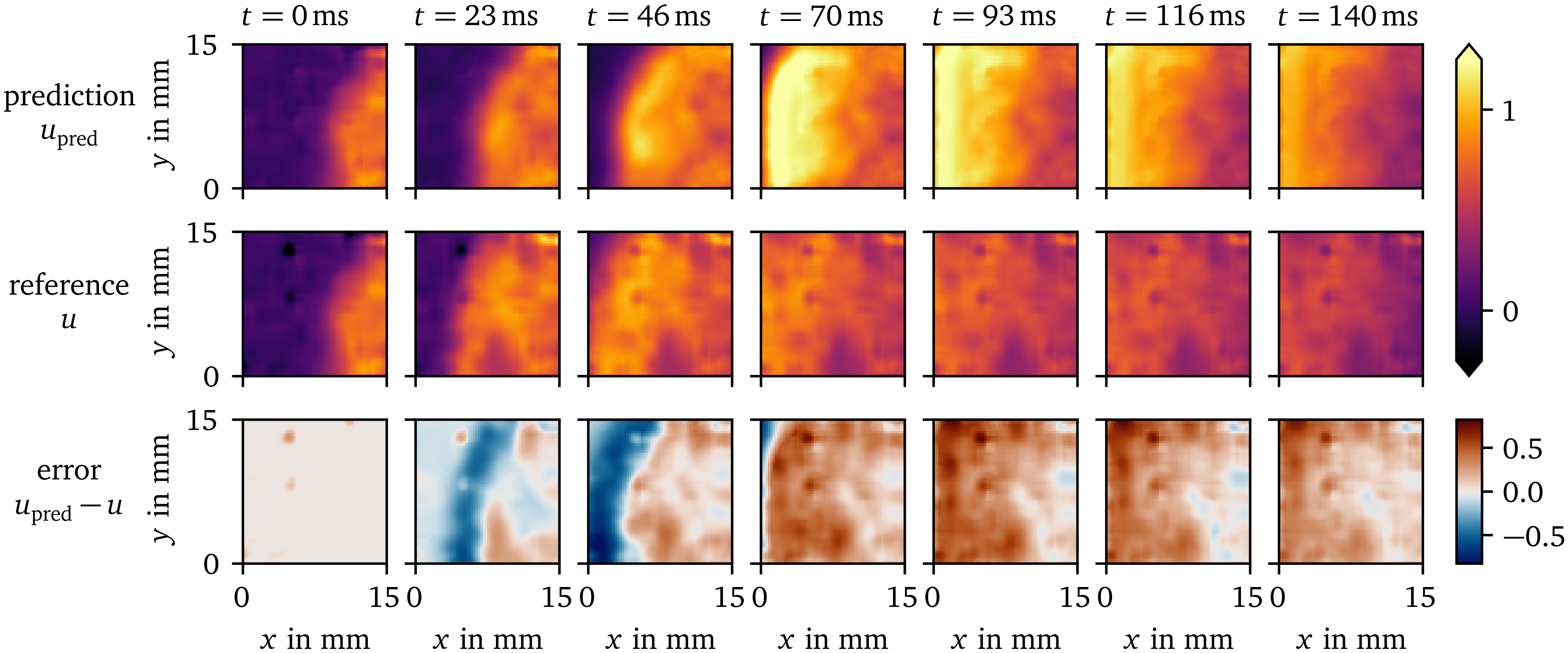
Figure 9: Prediction of the data-driven model over time compared to the reference solution for the OVM data set. The difference between the prediction and reference is displayed in the bottom row.
It can be seen that such artefacts due to inhomogeneity in the monolayer and other more complex effects are difficult to predict for the model, which only gets the state ${{\bm{{u}}}}{{\left( t_0, {{\bm{{x}}}} \right)}}$ at the initial time as input. Yet, similar structures are found in the prediction.
For the OVM data, the repolarisation at the wave back is much slower than the depolarisation at the wave front. For the synthetic data set AP96 re- and depolarisation happen at roughly the same time scale. Still, the one EMA variable $\tilde u$ is enough to capture these processes in both cases.
Prediction of a spiral wave
In Fig. 10, we compare a rotor in another OVM recording of hiAMs and a rotor predicted by the in-silico data-driven model. The model has been fit to data from only focal waves. To stimulate a spiral wave, we use the rectangle-based initial conditions outlined in section 2.1.2. Like for the synthetic data set (AP96, section 3.1), the tissue model is able to predict the overall spiral dynamics. Note that the spiral wave in the OVM recording has stabilised for several minutes before $t={0~\mathrm{{m}{s}}}$, while the rotor is just forming in the simulation with the data-driven model. The APD predicted by the model is much longer than the one observed APD by OVM. This leads to the wave front running into the wave back in the simulation.
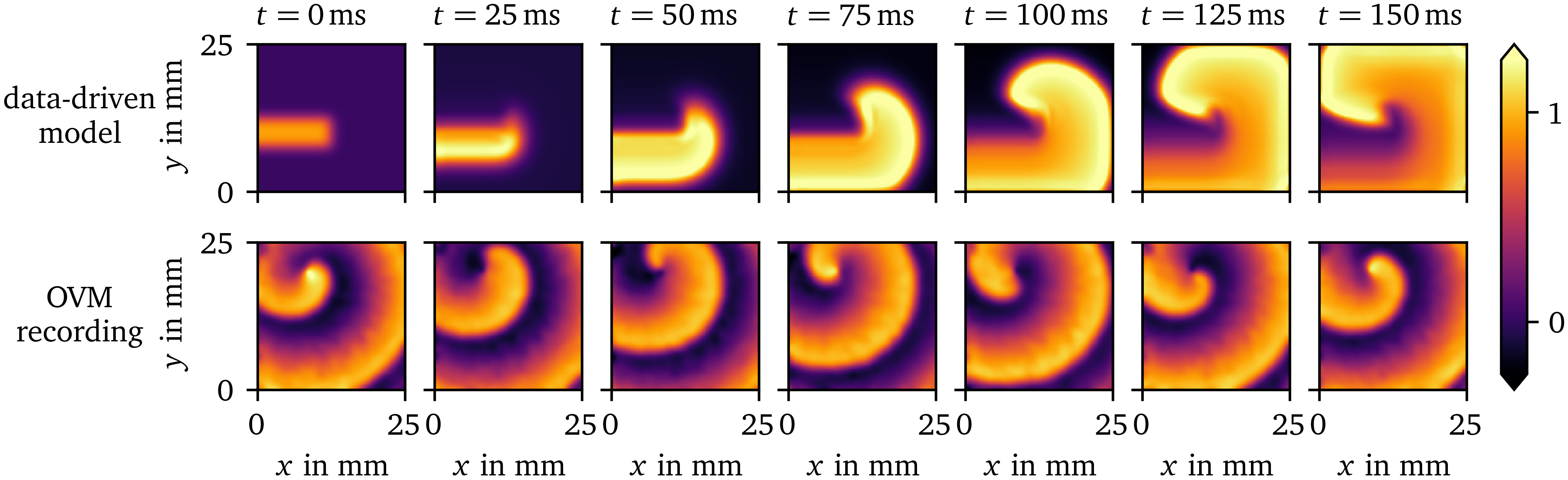
Figure 10: Comparison of a spiral wave for the data-driven model for the OVM data set for hiAMs to a OVM recording of hiAMs showing a stable rotor. The data-driven model can predict the overall dynamics of the spiral wave despite only focal waves being included in the training data it is fit to.
Discussion
In this paper, we have shown that enough information can be extracted from just one spatio-temporal variable to build a state space, which enables the creation of in-silico models that can predict the further dynamics of the system. In layman’s terms, from a single movie showing the behaviour of excitation and recovery, a predictive model can be constructed. Just the information from OVM is already enough to fit a data-driven model to the dynamics. With our approach, it is even possible to fit a stable model to a single excitation wave, which, in turn, does not generalise well to other waves. For this reason, the SBP protocol is designed to ensure that less likely stimulation patterns are observed in the data, too. The resulting models are able to replicate the excitation patterns of focal waves included in the training data and can even predict the dynamics of spiral waves, a pattern that the models are not trained on.
While the variables with which we augment the state space should be seen as preliminary and not optimal choices, the models created with these variables already are able to capture crucial behaviour of the tissue, namely excitation, recovery and wave propagation. Both short and long-term memory can be encoded with the use of EMAs as state variables, which can easily be updated on the fly (Eq. 7). It remains to be seen if more or other state space augmentations can be used to be able to replicate higher-order effects, such as wave front curvature and to obtain more accurate restitution behaviour.
Through state space expansion with EMAs and SDs, we have found a way to encode useful information to describe the mechanics of excitation waves. It is remarkable, that, after “unfolding” with the proper state space expansion, we are able to capture with simple polynomial regression the kinetics of excitation waves sufficiently in the sense that we observe excitation and recovery with an APD similar to the data, and wave propagation at a similar CV.
The polynomial model $f$ is fit using a basic supervised machine learning method. However, this is just a small part of the method presented in this work. We have shown that using unsupervised learning, i.e., data transformations, much insight can be gained about the structure of the data. The insights obtained from presenting the data sets in the chosen three-dimensional state spaces as done in this work make it almost trivial to fit the data-driven model to the data. Fitting a function in the chosen state space is easier to interpret than black box approaches common in machine learning.
We have chosen to use an advection-based description of the wave propagation. This is due to the computation of the diffusion term $\nabla \cdot {{\bm{{D}}}} \nabla u$ in Eq. 12 being quite sensitive to small variations in $u$ and hence less robust to noisy data. The absolute gradient ${{\left\lVert \nabla u \right\rVert}}$ as approximated using the SD $g$ can deal with noise much better by design. Solving the forward equations in the advection-regression framework requires less computational effort in forward simulations than most traditional in-silico models and other novel approaches utilising convolutional and physics-informed neural networks. In the numerical solution of reaction-diffusion systems (Eq. 12), a sufficiently small numerical time step must be chosen according to a stability criterion. Typically, this leads to numerical time steps of the order of magnitude in two-dimensional simulations of in-silico tissue models of cardiac electrophysiology. Forward Euler stepping our model in the advection-regression framework can be done at much larger time steps of up to with the trade-off of fitting less to the original data. Also the computation of the polynomial $f$, EMAs and SDs result in an overall computationally cheaper model than typical tissue models.
While this was not needed for this use case, in further research, more sophisticated general function approximators may be tried for $f$, such as neural networks. Although the Latin hypercube sampling enables some basic regularisation of the solution, it remains to be seen how to keep the fit functions simple enough such that they generalise well. Another limitation that could be addressed when using more flexible function approximators is that, in some cases, the polynomial model $f$ updates the state $u$ such that it tries to leave the valid range.
While other augmentations were tried in the development of this method, such as pseudo-electrograms, the last APD and diastolic interval at each point over time, or the absolute value of the gradient fit to a neighbourhood of each point using the least-squares method, we are here presenting two augmentations we found most useful, the EMA $\tilde u$ as well as the SD $g$.
We have not yet taken into account boundary effects in the model creation procedure. Some information about the gradient of the main variable $u$ is encoded in the SD $g$ in the neighbourhood of each point in the medium. The SD $g$ can still be computed near the boundary by treating those points just like interior points but with fewer samples. How to encode boundary conditions in this model could be investigated in follow-up studies.
The procedure to generate in-silico tissue models is designed to work well in a setting where not much is known about the wave propagation in an in-vitro tissue model. Our method only requires very little assumptions to uncover the dynamics. Fitting is not limited to just in-vitro OVM data of focal waves in cardiac tissue excitation models, but can also be done in general where excitation wave dynamics can be observed in two dimensional space over time. An advantage of our method is that models for any observed behaviour can be created and fit to data which is in contrast to classical phenomenological models (Aliev & Panfilov, 1996; Barkley, 1991; Bueno-Orovio et al., 2008; Fenton & Karma, 1998; FitzHugh, 1961; Marcotte & Grigoriev, 2017; Nagumo et al., 1962). Fitting parameters of such existing models can get the model closer to observed data. However, if a behaviour falls outside the regime of these models, such methods will not work (Martin et al., 2022). With our method, a data-driven model can be fit flexibly with relative ease within minutes and subsequently used to predict the further evolution of the tissue. This puts our model creation pipeline more in line with recent deep learning approaches (Costabal et al., 2020; Martin et al., 2022; Shahi et al., 2022). However, our approach is typically faster in fitting due to the polynomial model function and faster in forward stepping because of the SD-based spatial coupling. Depending on the complexity of the dynamics, a simple approach to modelling such as ours may be enough. Promising use cases to apply the proposed method with minimal changes are the peristaltic motion of for instance embryonic hearts or the digestive tract (Moorman & Christoffels, 2003), or the spread of lichens which has been observed to form spiral waves (Müller & Tsuji, 2019). For more complex dynamics, more than three state space variables may be needed, or an extension using a neural network as the model function $f$. For very complex dynamics, the aforementioned, more extensive deep learning methods may be necessary (Aliev & Panfilov, 1996; Barkley, 1991; Bueno-Orovio et al., 2008; Fenton & Karma, 1998; FitzHugh, 1961; Marcotte & Grigoriev, 2017; Nagumo et al., 1962). Possible extensions of our data-driven model include an online-learning approach, where the model’s predictive power is continuously improved while new data comes in. Such a model could, for instance, be fit to patient recordings, such as intra-cardiac electrograms or electrocardiograms on the body surface, and then be used to predict cardiac arrhythmias before they happen.
Conclusion
In this work, we presented a method to create simple data-driven in-silico tissue models from in-vitro OVM data and synthetic data that capture the basic behaviour of the corresponding excitable media. These models can predict the activation patterns included in the training data, i.e., only focal waves, and generalise to unseen activation patterns, such as spiral waves. A useful feature of this model creation method is its ability to extract all relevant information that the models are fit to from just one state variable over space and time, such as the transmembrane voltage of cardiomyocytes which can be obtained from a single experiment, e.g. an OVM recording.
Data availability
The source code of the software implemented for this paper is publicly available at https://gitlab.com/heartkor. The functionality is broken up into several separate packages, some of which depend on each other.
The model creation pipeline is implemented as the Distephym Python
module, distephym 1.0.0. It
stores the augmented state spaces in sparse histograms, specifically
implemented for this publication as another module,
sparsealgos 1.0.0.
Reading, writing, and analysis of OVM recordings is implemented in the
Sappho Python module,
sappho 1.0.0.
The Ithildin C++ framework,
ithildin 3.2.2, is a
finite-differences, parallelised, reaction-diffusion solver written in
C++. It will be released in a separate, dedicated publication (Cloet et
al., 2023; Kabus et al.,
2024). We have used Ithildin to generate the
synthetic (i.e., AP96) data set.
For the other forward simulations in this work, we have written another
simple finite-differences reaction-diffusion solver in Python,
ithilmin 1.0.0, that can
easily be combined with other Python modules. It was used for forward
runs of the fit data-driven models.
In conjunction with this paper, we are also releasing a new version of
the Ithildin Python module,
py_ithildin 0.6.1, (Kabus
et al., 2022). This module was used for the
processing of in-vitro/in-silico data sets. Results from both
reaction-diffusion solvers, ithildin and ithilmin, can be analysed
with this Python module.
The source code of these projects and the AP96 and OVM data sets used in this work have been archived on Zenodo (DOI: 10.5281/zenodo.8183722).
Addenda
Acknowledgments:
We are grateful to our collaborators at the LUMC, especially to Sven O. Dekker and Juan Zhang for providing access to hiAM monolayers and the OVM setup, and to Niels Harlaar for the spiral wave OVM recordings, respectively. Also, we would like to thank all members of Team HeartKOR at KULAK for valuable help during writing, in particular, Marie Cloet.
Funding:
DK is supported by KU Leuven grant GPUL/20/012. HD is supported by KU Leuven grant STG/19/007. The funders had no role in study design, data collection and analysis, decision to publish, or preparation of the manuscript. The hiAMs were developed as part of the research programme “More Knowledge with Fewer Animals” (MKMD, project 114022503, to AAFdV), which was financed by the Netherlands Organisation for Health Research and Development (ZonMw) and by the Dutch Society for the Replacement of Animal Testing (dsRAT).
Competing interests:
The authors have declared that no competing interests exist.
Copyright:
© 2024 The Authors. Published by Elsevier Ltd. This is an open access article under the CC BY license (http://creativecommons.org/licenses/by/4.0/).
Author contributions:
DK: Conceptualisation, Methodology, Software, Validation, Formal analysis, Investigation, Data curation, Writing – original draft, Writing – review & editing, Visualisation. TDC: Methodology, Writing – review & editing. AAFdV: Conceptualisation, Resources, Writing – review & editing. DAP: Conceptualisation, Resources, Writing – review & editing, Supervision, Project administration, Funding acquisition. HD: Conceptualisation, Resources, Writing – review & editing, Supervision, Project administration, Funding acquisition.
References
Aliev, R. R., & Panfilov, A. V. (1996). A simple two-variable model of cardiac excitation. Chaos, Solitons & Fractals, 7(3), 293–301. https://doi.org/10.1016/0960-0779(95)00089-5
Barkley, D. (1991). A model for fast computer simulation of waves in excitable media. Physica D: Nonlinear Phenomena, 49(1-2), 61–70. https://doi.org/10.1016/0167-2789(91)90194-e
Bayly, P. V., KenKnight, B. H., Rogers, J. M., Hillsley, R. E., Ideker, R. E., & Smith, W. M. (1998). Estimation of conduction velocity vector fields from epicardial mapping data. IEEE Transactions on Biomedical Engineering, 45(5), 563–571. https://doi.org/10.1109/10.668746
Bressloff, P. C. (2014). Waves in neural media. Lecture Notes on Mathematical Modelling in the Life Sciences, 18–19. https://doi.org/10.1007/978-1-4614-8866-8
Bueno-Orovio, A., Cherry, E. M., & Fenton, F. H. (2008). Minimal model for human ventricular action potentials in tissue. Journal of Theoretical Biology, 253(3), 544–560. https://doi.org/10.1016/j.jtbi.2008.03.029
Clayton, R., Bernus, O., Cherry, E. M., Dierckx, H., Fenton, F. H., Mirabella, L., Panfilov, A. V., Sachse, F. B., Seemann, G., & Zhang, H. (2011). Models of cardiac tissue electrophysiology: Progress, challenges and open questions. Progress in Biophysics and Molecular Biology, 104(1-3), 22–48. https://doi.org/10.1016/j.pbiomolbio.2010.05.008
Cloet, M., Arno, L., Kabus, D., Van der Veken, J., Panfilov, A. V., & Dierckx, H. (2023). Scroll waves and filaments in excitable media of higher spatial dimension. Physical Review Letters, 131(20), 208401. https://doi.org/10.1103/PhysRevLett.131.208401
Costabal, F. S., Yang, Y., Perdikaris, P., Hurtado, D. E., & Kuhl, E. (2020). Physics-informed neural networks for cardiac activation mapping. Frontiers in Physics, 8. https://doi.org/10.3389/fphy.2020.00042
Courtemanche, M., Ramirez, R. J., & Nattel, S. (1998). Ionic mechanisms underlying human atrial action potential properties: Insights from a mathematical model. American Journal of Physiology-Heart and Circulatory Physiology, 275(1), H301–H321. https://doi.org/10.1152/ajpheart.1998.275.1.H301
Fenton, F. H., & Karma, A. (1998). Vortex dynamics in three-dimensional continuous myocardium with fiber rotation: Filament instability and fibrillation. Chaos: An Interdisciplinary Journal of Nonlinear Science, 8(1), 20–47. https://doi.org/10.1063/1.166311
FitzHugh, R. (1961). Impulses and physiological states in theoretical models of nerve membrane. Biophysical Journal, 1(6), 445–466. https://doi.org/10.1016/s0006-3495(61)86902-6
Fox, J. J., Bodenschatz, E., & Gilmour, R. F. (2002). Period-doubling instability and memory in cardiac tissue. Physical Review Letters, 89(13). https://doi.org/10.1103/physrevlett.89.138101
Gillette, K., Gsell, M. A. F., Prassl, A. J., Karabelas, E., Reiter, U., Reiter, G., Grandits, T., Payer, C., Štern, D., Urschler, M., Bayer, J. D., Augustin, C. M., Neic, A., Pock, T., Vigmond, E. J., & Plank, G. (2021). A framework for the generation of digital twins of cardiac electrophysiology from clinical 12-leads ECGs. Medical Image Analysis, 71, 102080. https://doi.org/10.1016/j.media.2021.102080
Gray, R. A., Jalife, J., Panfilov, A. V., Baxter, W. T., Cabo, C., Davidenko, J. M., & Pertsov, A. M. (1995). Mechanisms of cardiac fibrillation. Science, 270(5239), 1222–1223. https://doi.org/10.1126/science.270.5239.1222
Harlaar, N., Dekker, S. O., Zhang, J., Snabel, R. R., Veldkamp, M. W., Verkerk, A. O., Fabres, C. C., Schwach, V., Lerink, L. J. S., Rivaud, M. R., Mulder, A. A., Corver, W. E., Goumans, M. J. T. H., Dobrev, D., Klautz, R. J. M., Schalij, M. J., Veenstra, G. J. C., Passier, R., Brakel, T. J. van, Pijnappels, D. A., & Vries, A. A. F. de. (2022). Conditional immortalization of human atrial myocytes for the generation of in vitro models of atrial fibrillation. Nature Biomedical Engineering, 6(4), 389–402. https://doi.org/10.1038/s41551-021-00827-5
Joukar, S. (2021). A comparative review on heart ion channels, action potentials and electrocardiogram in rodents and human: Extrapolation of experimental insights to clinic. Laboratory Animal Research, 37(1), 1–15. https://doi.org/10.1186/s42826-021-00102-3
Kabus, D., Arno, L., Leenknegt, L., Panfilov, A. V., & Dierckx, H. (2022). Numerical methods for the detection of phase defect structures in excitable media. PLOS ONE, 17(7), 1–31. https://doi.org/10.1371/journal.pone.0271351
Kabus, D., Cloet, M., Zemlin, C., Bernus, O., & Dierckx, H. (2024). The Ithildin library for efficient numerical solution of anisotropic reaction-diffusion problems in excitable media. PLOS ONE, 19(9), 1–26. https://doi.org/10.1371/journal.pone.0303674
Krogh-Madsen, T., Schaffer, P., Skriver, A. D., Taylor, L. K., Pelzmann, B., Koidl, B., & Guevara, M. R. (2005). An ionic model for rhythmic activity in small clusters of embryonic chick ventricular cells. American Journal of Physiology-Heart and Circulatory Physiology, 289(1), H398–H413. https://doi.org/10.1152/ajpheart.00683.2004
Kuklik, P., Zeemering, S., Maesen, B., Maessen, J., Crijns, H. J., Verheule, S., Ganesan, A. N., & Schotten, U. (2014). Reconstruction of instantaneous phase of unipolar atrial contact electrogram using a concept of sinusoidal recomposition and hilbert transform. IEEE Transactions on Biomedical Engineering, 62(1), 296–302. https://doi.org/10.1109/TBME.2014.2350029
Majumder, R., Jangsangthong, W., Feola, I., Ypey, D. L., Pijnappels, D. A., & Panfilov, A. V. (2016). A mathematical model of neonatal rat atrial monolayers with constitutively active acetylcholine-mediated k+ current. PLoS Computational Biology, 12(6), e1004946. https://doi.org/10.1371/journal.pcbi.1004946
Marcotte, C. D., & Grigoriev, R. O. (2017). Dynamical mechanism of atrial fibrillation: A topological approach. Chaos: An Interdisciplinary Journal of Nonlinear Science, 27(9). https://doi.org/10.1063/1.5003259
Martin, C. H., Oved, A., Chowdhury, R. A., Ullmann, E., Peters, N. S., Bharath, A. A., & Varela, M. (2022). EP-PINNs: Cardiac electrophysiology characterisation using physics-informed neural networks. Frontiers in Cardiovascular Medicine, 8. https://doi.org/10.3389/fcvm.2021.768419
McKay, M. D., Beckman, R. J., & Conover, W. J. (2000). A comparison of three methods for selecting values of input variables in the analysis of output from a computer code. Technometrics, 42(1), 55–61. https://doi.org/10.1080/00401706.2000.10485979
Moe, G. K., Rheinbolt, W. C., & Abildskov, J. A. (1964). A computer model of atrial fibrillation. Am. Heart J., 67, 200–220. https://doi.org/10.1016/0002-8703(64)90371-0
Moorman, A. F. M., & Christoffels, V. M. (2003). Cardiac chamber formation: Development, genes, and evolution. Physiological Reviews. https://doi.org/10.1152/physrev.00006.2003
Müller, S. C., & Tsuji, K. (2019). Appearance in nature. Spirals and Vortices: In Culture, Nature, and Science, 31–66. https://doi.org/10.1007/978-3-030-05798-5_2
Nagumo, J., Arimoto, S., & Yoshizawa, S. (1962). An active pulse transmission line simulating nerve axon. Proceedings of the IRE, 50(10), 2061–2070. https://doi.org/10.1109/jrproc.1962.288235
Niederer, S. A., Lumens, J., & Trayanova, N. A. (2019). Computational models in cardiology. Nature Reviews Cardiology, 16(2), 100–111. https://doi.org/10.1038/s41569-018-0104-y
Noble, J. V. (1974). Geographic and temporal development of plagues. Nature, 250(5469), 726–729. https://doi.org/10.1038/250726a0
O’Hara, T., & Rudy, Y. (2012). Quantitative comparison of cardiac ventricular myocyte electrophysiology and response to drugs in human and nonhuman species. American Journal of Physiology-Heart and Circulatory Physiology, 302(5), H1023–H1030. https://doi.org/10.1152/ajpheart.00785.2011
Paci, M., Hyttinen, J., Aalto-Setälä, K., & Severi, S. (2013). Computational models of ventricular-and atrial-like human induced pluripotent stem cell derived cardiomyocytes. Annals of Biomedical Engineering, 41(11), 2334–2348. https://doi.org/10.1007/s10439-013-0833-3
Priebe, L., & Beuckelmann, D. J. (1998). Simulation study of cellular electric properties in heart failure. Circulation Research, 82(11), 1206–1223. https://doi.org/10.1161/01.res.82.11.1206
Shahi, S., Fenton, F. H., & Cherry, E. M. (2022). A machine-learning approach for long-term prediction of experimental cardiac action potential time series using an autoencoder and echo state networks. Chaos: An Interdisciplinary Journal of Nonlinear Science, 32(6). https://doi.org/10.1063/5.0087812
ten Tusscher, K. H. W. J., Noble, D., Noble, P.-J., & Panfilov, A. V. (2004). A model for human ventricular tissue. American Journal of Physiology-Heart and Circulatory Physiology, 286(4), H1573–H1589. https://doi.org/10.1152/ajpheart.00794.2003
Trayanova, N. A., Doshi, A. N., & Prakosa, A. (2020). How personalized heart modeling can help treatment of lethal arrhythmias: A focus on ventricular tachycardia ablation strategies in post‐infarction patients. WIREs Systems Biology and Medicine, 12(3). https://doi.org/10.1002/wsbm.1477
Wei, N., Mori, Y., & Tolkacheva, E. G. (2015). The role of short term memory and conduction velocity restitution in alternans formation. Journal of Theoretical Biology, 367, 21–28. https://doi.org/10.1016/j.jtbi.2014.11.014